
Recommended
Recommended
More Related Content
What's hot
What's hot (20)
Viewers also liked
Viewers also liked (20)
Similar to Woodward hall entrepreneurship aer 2010
Similar to Woodward hall entrepreneurship aer 2010 (20)
Recently uploaded
Recently uploaded (20)
Woodward hall entrepreneurship aer 2010
- 1. The Burden of the Nondiversifiable Risk of Entrepreneurship By Robert E. Hall and Susan E. Woodward∗ Entrepreneurship is risky. We study the risk facing a well-documented and important class of entrepreneurs, those backed by venture capital. Using a dynamic program, we calculate the certainty-equivalent of the difference between the cash rewards that entrepreneurs actually received over the past 20 years and the cash that entrepreneurs would have received from a risk-free salaried job. The payoff to a venture-backed entrepreneur comprises a below-market salary and a share of the equity value of the company when it goes public or is acquired. We find that the typical venture-backed entrepreneur received an average of $5.8 million in exit cash. Almost three-quarters of entrepreneurs receive nothing at exit and a few receive over a billion dollars. Because of the extreme dispersion of payoffs, an entrepreneur with a coefficient of relative risk aversion of two places a certainty-equivalent value only slightly greater than zero on the distribution of outcomes she faces at the time of her company’s launch. (JEL: ) An entrepreneur’s primary incentive is ownership of a substantial share of the enter- prise that commercializes the entrepreneur’s ideas. An inescapable consequence of this incentive is the entrepreneur’s exposure to the idiosyncratic risk of the enterprise. Diver- sification or insurance to ameliorate the risk would necessarily weaken the incentives for success. We study this issue in the case of startup companies backed by venture capital. These startups are mainly in information technology and biotechnology. They harness teams comprising entrepreneurs (scientists, engineers, and executives), venture capitalists (gen- eral partners of venture funds), and the suppliers of capital (the limited partners of ven- ture funds). During the startup process, entrepreneurs collect only sub-market salaries. The compensation that attracts them to startups is the share they receive of the value of a company if it goes public or is acquired. We make use of a rich body of data, which covers close to the universe of companies receiving venture funding from 1987 to 2008, though some information is missing for many companies. We use a method for imputing missing data that takes account of selection bias. Our most important finding is that the reward to the entrepreneurs who provide the ideas and long hours of hard work in these startups is zero in almost three quarters of the outcomes, and small on average once idiosyncratic risk is taken into consideration. Standard venture deals involve three parties—entrepreneurs, general partners, and lim- ited partners. The entrepreneurs have leveraged positions; that is, they receive no payoff until other claimants have received prescribed payoffs. The general partners, who arrange ∗ Hall: Hoover Institution and Department of Economics, Stanford University (email: re- hall@stanford.edu); Woodward: Sandhill Econometrics, 115 Everett Street, Palo Alto, CA 94301 (email: swoodward@sandhillecon.com). We are grateful to the referees, Ravi Jagannathan, Deborah Lucas, Matthew Rhodes-Kropf, and numerous seminar participants for comments and to Katherine Litvak for data on venture-contract terms. Hall’s research is part of the Economic Fluctuations and Growth Pro- gram of the National Bureau of Economic Research. 1
- 2. 2 THE AMERICAN ECONOMIC REVIEW DECEMBER 2009 financing and supervise the startup company by holding board seats, are compensated in proportion to the amount invested and the capital gains from the investment. The limited partners are passive investors who hold debt and equity claims on the startup. General partners are somewhat diversified across investments and the limited partners are highly diversified. The burden of specialization falls mainly on the entrepreneurs. Robert E. Hall and Susan E. Woodward 2007 describes the returns to the general partners and limited partners. This paper deals exclusively with the entrepreneurs. Although the average ultimate cash reward to an entrepreneur in a company that suc- ceeds in landing venture funding is $5.8 million, most of this expected value comes from the small probability of a great success. An individual with a coefficient of relative risk aversion of 2 and assets of $188,949 is indifferent between employment at a market salary and entrepreneurship. With lower risk aversion or higher initial assets, the entrepreneurial opportunity is worth more than alternative employment. We infer that entrepreneurs are drawn differentially from individuals with lower risk aversion and higher assets. Other types of people that may be attracted to entrepreneurship are those with preferences for that role over employment and those who exaggerate the likely payoffs of their own prod- ucts. Our model does not include these factors, however—we use standard preferences based on consumption levels alone. We focus on the joint distribution of the duration of the entrepreneur’s involvement in a startup—what we call the venture lifetime—and the value that the entrepreneur receives when the company exits the venture portfolio. Exits take three forms: (1) an initial public offering, in which the entrepreneur receives liquid publicly-traded shares 6 months after the IPO and has the opportunity to diversify; (2) the sale of the company to an acquirer, in which the entrepreneur receives cash or publicly-traded shares in the acquiring company and has the opportunity to diversify; and (3) shutdown or other determination that the entrepreneur’s equity interest has essentially no value. Most IPOs return substantial value to an entrepreneur. Some acquisitions also return substantial value, while others may deliver a meager or zero value. The joint distribution shows a distinct negative correlation between exit value and venture lifetime. Highly successful products tend to result in IPOs or acquisitions at high values relatively quickly. These outcomes are favorable for entrepreneurs in two ways. First, the value arrives quickly and is subject to less discounting. Second, the entrepreneur spends less time being paid a low startup salary and correspondingly more time with higher post-startup compensation, in the public version of the original company, in the acquiring company, or in another job. A fraction of entrepreneurs launch new startups after exiting from an earlier startup. Throughout the paper, we study exit values from the point of view of the individ- ual entrepreneur. About a quarter of entrepreneurs do not share the proceeds with other entrepreneurs; they operate solo. Another quarter share the entrepreneurial role equally with another founder. In the remaining cases, entrepreneurial ownership is dis- tributed asymmetrically between a pair of entrepreneurs or there are three or even more entrepreneurs. We measure the total entrepreneurial return delivered by each venture company and then infer the returns to the individual entrepreneurs from information about the distribution among entrepreneurs. All of the tabulations in the paper refer to entrepreneurs, not to companies. We develop a unified analysis of the factors affecting the entrepreneur’s risk-adjusted payoff, based on a dynamic program. The analysis takes account of the joint distribution of exit value and venture lifetime and of salary and compensation income. We use it to calculate the certainty-equivalent value of the entrepreneurial opportunity—the amount that a prospective entrepreneur would be willing to pay to become a founder of a venture- backed startup. For a risk-neutral individual, the certainty-equivalent is $5.8 million.
- 3. VOL. 99 NO. 6 RISK OF ENTREPRENEURSHIP 3 With mild risk aversion and savings of $100,000, however, the amount is only $0.6 million and with normal risk aversion and that amount of savings, the certainty-equivalent is slightly negative. We are not aware of any earlier research that quantifies the rewards on a per-company basis or per-entrepreneur-year basis, the focus of our work. Earlier research on venture- backed startups has focused on the returns to venture investors. An extensive theo- retical literature considers the implications of idiosyncratic risk for entrepreneurs and managers—see John Heaton and Deborah Lucas 2004 for a recent contribution and many references. I. What This Paper Does Our first step is the development of data for the great majority of all venture-backed startups in the U.S. from the date of each one’s first venture funding, covering subsequent venture fundings, the date of exit, and the cash payoff to the entrepreneurs as a group. We start by determining the founding equity interest of the entrepreneurs, then track the dilution of the entrepreneurs’ interest through successive rounds of venture investment. We take account of extra dilution mandated by the standard venture contract if a later round of investment places a lower value on the company than did an earlier round—a “down round.” We calculate the entrepreneurs’ share of the proceeds from an exit. Here we take account of the debt aspects of the venture investors’ claims on the company, the preferences associated with their holdings. Successful exits are IPOs or high-priced acqui- sitions by another company; unsuccessful ones are shutdowns and low-price acquisitions in which the entrepreneurs receive nothing. The output from the first step is the starting date, exit date, and combined exit value for the entrepreneurs in each of the companies. The next step develops tabulations of the joint distribution of venture lifetime—the time from startup to exit—and exit values for individual entrepreneurs, based on data for entrepreneurs’ group exit values and data on the distribution of individual entrepreneurs’ shares among the total equity holdings of the entrepreneurs as a group. The third step constructs a personal financial model of the entrepreneur during the startup experience. The model captures the implications of the idiosyncratic risk facing the entrepreneur. No insurance is available to deal with the risk. Rather, the entrepreneur works for an uncertain number of years at a sub-market salary and may or may not receive an exit value somewhere between a few hundred thousand dollars and a billion dollars. The model considers both elements of risk—the number of years of foregone earnings and the uncertainty about the payoff. II. The Startup Process At the outset, startups are usually operated and financed by the entrepreneurs them- selves. Friends and family may invest as founding shareholders. Unless the founders are wealthy, they need outside financing, so a main task early in a startup is to find investors. Some are individual investors called angels. But venture funds are capable of investing more at the outset than is available from these other sources, and venture can invest large amounts later in the development of a startup with a promising product. Our concern is with the companies that succeed in obtaining venture funding by convincing some venture capitalists that the new business has a positive net present value, which, given the skewness of the distribution of value at outcome, implies at least some chance of becoming highly profitable. Venture funds seldom give a company all of the money it will need to get from startup to exit in a single investment. Instead, a syndicate of venture funds will provide financing in rounds, anticipating future rounds of funding, possibly including different investors,
- 4. 4 THE AMERICAN ECONOMIC REVIEW DECEMBER 2009 if the startup makes reasonable progress but still lacks the revenue to be self-sustaining, and denying the startup further funding otherwise. An early round typically gives a startup a few million dollars, while later rounds, if they occur, often involve much larger investments. General partners are the organizers of venture funds. They recruit financing commit- ments from limited partners—usually pension funds, endowments, and wealthy individuals— and choose the companies that will receive financing. Compensation to general partners comprises an annual fraction of two to three percent of the limited partners’ invested cap- ital plus carry—20 to 30 percent of the profit from successful exits. The limited partners receive most of the cash returned by venture investments when a company undergoes a favorable exit event—an IPO or acquisition. Venture funds generally hold convertible preferred shares in their portfolio companies. The preference requires that the funds receive a specified amount of cash back before the common shareholders (the entrepreneurs, angels, and employees) receive any return. In a successful outcome, the convertible preferred shares convert shares to common stock. Instead of convertible preferences, venture funds may hold debt claims, in which case they receive the repayment of the debt even in the best outcomes. Both arrangements put the common shareholders, including the entrepreneurs, in a leveraged position, increasing their exposure to the idiosyncratic risk of the startup. A huge literature portrays the standard venture financial contract as the constrained optimum of a challenging mechanism design problem. This research explains key features, including the assignment of a share of the ultimate value to the entrepreneurs, multiple stages of financing, and debt instruments (preferences) that convert to equity. Some of the more prominent contributions include Anat R. Admati and Paul Pfleiderer 1994, Klaus M. Schmidt 2003, Catherine Casamatta 2003, and Rafael Repullo and Javier Suarez 2004. Alex Wilmerding 2003 and Constance E. Bagley and Craig E. Dauchy 2003 explain the terms of venture contracts from the perspective of venture capitalists and their lawyers. The dominant factor in this literature is moral hazard. Venture investors and their agents, the general partners of venture funds, are unable to monitor or specify the efforts of entrepreneurs to commercialize their ideas. Consequently, the entrepreneurs are paid in proportion to the actual commercial success of their companies. This alignment of incentives comes at the cost of a substantial diminution in the value of the enterprise because of the idiosyncratic risk that entrepreneurs are unable to insure. Alternatives with less risk, such as paying entrepreneurs salaries in place of equity, apparently pro- vide such weak incentives that the relationship based on equity incentives weakened by idiosyncratic risk is still optimal for some products and some entrepreneurs. Venture capitalists face a daunting problem evaluating proposals for startups. One of the reasons that entrepreneurs receive sub-market salaries during the startup phase is to induce self-selection among applicants for venture funding. Only entrepreneurs with confidence in the commercial values of their ideas will seek funding if the entrepreneur’s payoff from an unsuccessful startup is negative. Most of the expected return to entrepreneurs comes from low-probability large gains. About three-quarters of venture-backed companies expire without returning any cash to their entrepreneurs. The largest returns generally come from IPOs, but acquisitions sometimes provide high returns as well. On the other hand, many acquisitions occur at low prices and are effectively liquidations. Some venture-backed companies remain for many years as stand-alone operations, able to pay their employees out of revenue, but generating no returns for shareholders. The free-standing startup company is one of the ways that ideas for new products are developed and marketed. It provides powerful incentives for its entrepreneurs, but at the cost of exposing them to the idiosyncratic risks of their companies. Most scientists and
- 5. VOL. 99 NO. 6 RISK OF ENTREPRENEURSHIP 5 engineers working on new products work as employees for established—often very large— companies. Their employment contracts isolate them from the most of the idiosyncratic risks of the products they develop. Incentives are not as powerful as in startups. We discuss the sorting of potential entrepreneurs into startups and established companies in a concluding section. We note that the market for scientists and engineers has not developed any intermediate contract, though one could imagine such a contract. It would pay a higher salary than the standard venture contract does, but provide less exit value, for example, by putting a ceiling on the payout. We believe that such contracts are rare. The two successful contract forms in the market for technical talent are polar opposites. The intermediate contract appears not to be viable. III. Data A. Data on venture transactions We use a database compiled by Sand Hill Econometrics on venture investments in startups and on the fates of venture-backed companies. The data are drawn from a variety of sources, including several commercial data vendors. A comparison of the list of companies in the database to lists of companies in pension plan venture investments, shows that the Sand Hill data includes close to the universe of venture-funded startups from 1987 to the present. The data vendors concentrate on reporting funding events and valuations for venture investments and successful outcomes (IPOs and high-value acquisitions) and are less likely to report shutdowns and acquisitions at low values. Sand Hill Econometrics has used a wide range of sources to augment coverage of these adverse termination events. The Data Appendix posted in the archives of this journal and on the first author’s website describes the data in more detail and documents the technique we use to track the evolution of the entrepreneurs’ ownership of a company through successive rounds of funding, each of which dilutes the entrepreneurs’ claims. Our measurement of the entrepreneur’s take from the exit value of the enterprise starts with the total cash received by the owners collectively. In the case of an IPO, this amount is the total market value of the newly public company less the cash raised in the IPO. For an acquisition, it is the total amount paid to the shareholders of the company. We divide this amount among the owners in the way specified in the standard venture contracts between the venture capitalist and shareholders. Immediately prior to the first venture investment, the entrepreneurs own most of the enterprise. The other shareholders are usually angels—individual investors—and friends and family. We assume that the cash investments from the entrepreneurs are made prior to the first round of venture investments. As the development of the company progresses, the entrepreneurs’ ownership share declines. The main reason is that each round of venture investment purchases equity and debt claims that dilute the entrepreneur. In addition, the typical startup hires professional managers who receive stock options that convert to share ownership upon a remunerative exit event. For initial shares owned by angels, friends-and-family, and executives, we use data from published studies that report averages across venture-backed startups. For dilution from venture investments, we use data specific to each company based on round-by-round data from the Sand Hill database. Each round of venture financing purchases equity and debt claims on the startup. The debt claims take the form of preferences—cash due to venture investors upon an exit event on top of their equity claims. Some preferences pay off only in the poorer outcomes while others pay off in all outcomes. We apply standard formulas from venture contracts to estimate the deductions from entrepreneurial receipts resulting from preferences. The new equity issued in a round dilutes the ownership shares of the entrepreneurs. For
- 6. 6 THE AMERICAN ECONOMIC REVIEW DECEMBER 2009 investment rounds where the purchase price of the new shares—and thus the current value of all shares—are reported in the database, the dilution calculation is straightforward. Where the purchase price is not reported, we estimate the share of the company’s equity purchased in the round by the investors using a body of data suited to solving the sample selection problem. Another feature of the standard venture contract is anti-dilution protection to venture investors from earlier rounds if a later round assigns a lower value to the company. This protection shifts ownership from the entrepreneurs to the earlier venture investors to eliminate or ameliorate the decline in value they would otherwise suffer from a so-called down round. One important source of valuation data is S-1 statements filed by venture-backed com- panies when they go public. These statements often give a funding history for the com- pany. Because an IPO is a favorable event, the back-filling of round values from S-1s is a source of return-based selection in the data. The Appendix describes how we adjust for selection bias. Our data include 22,004 venture-backed companies, the great majority of all such companies in the United States for the period from the beginning of 1987 through the third quarter of 2008. Among the exit values used in the analysis, 2,015 are IPOs, 5,625 are acquisitions, and 3,352 are confirmed zero-value exits. Of the remaining companies, we treat those more than 5 years past their last rounds of venture funding as having exited at some time with zero value; 4,220 companies fall into this category. We randomly assign these companies exit dates by drawing from the empirical distribution of time past funding of companies with known zero-value exit dates. The remaining 6,792 companies have not yet achieved their exit values. For acquisitions, we use the reported exit value and exit date as the entrepreneur’s payoff, as we believe that lags in payments to entrepreneurs are quite brief. For IPOs, we assume that entrepreneurs are required to retain all of their publicly traded shares for a lockup period of six months, so we date the receipt of cash at 6 months past the IPO and the amount as the market value of the entrepreneurs’ holdings at that date. We state all exit values in 2006 dollars using the Consumer Price Index. Finally, we use the NBER TAXSIM model (http://www.nber.org/∼taxsim) to calcu- late the after-tax value of the cash received by an entrepreneur by applying the marginal tax rate on long-term capital gains to the entrepreneur’s exit cash, under U.S. and Cali- fornia income taxation (the majority of the entrepreneurs in the sample live in California). The rate is very close to 25 percent at all relevant levels of salary and capital gains in- come. We use 25 percent in all cases. We also use TAXSIM to calculate the after-tax values of the venture and alternative salaries. We consider pre-tax salaries of $150,000, $300,000, $600,000, and $2,000,000, which correspond to $111,220 , $194,126 , $367,212 , and $1,128,001 , after tax. We use 2006 tax rates, which are essentially the same as the rates for other recent years. B. Share of ownership by individual entrepreneur We use a model of personal or family decision making, where consumption depends on the earnings and exit values of individuals. Our data treat all the entrepreneurs in a company as a group. Our basic data sources do not contain information about the ownership shares of the individual entrepreneurs in each startup company. We use estimates from a sample of companies that underwent IPOs. The sample is a random draw of 100 candidates from all IPOs reported in our data. The SEC form S-1 filed prior to an IPO often contains a description of the major shareholders, which includes the entrepreneurs. The sample contains 41 companies and 66 entrepreneurs. Because the venture IPO sample is not necessarily representative of venture-backed startups in general,
- 7. VOL. 99 NO. 6 RISK OF ENTREPRENEURSHIP 7 we regard it as illustrative and far from definitive. We see little benefit from extending the sample to a larger number of IPOs. Our results are not at all sensitive to the method for restating company-based distributions as entrepreneur-based distributions. Table 1 describes the venture IPO sample. Just under a quarter of entrepreneurs receive all of the entrepreneurial exit value—these are solo entrepreneurs. At the other end, about a sixth of entrepreneurs receive less than 20 percent of the exit values of their companies. The right-hand column of the table shows the exit value of all of the entrepreneurs averaged across all companies that contain an entrepreneur in the share category corresponding to the row in the table. A solo entrepreneur, in the bottom line of the table, receives all of an average of $91 million of exit value, while an entrepreneur with less than a 20-percent share receives less than a fifth of an average of $48 million of exit value. There appears to be a positive relation between an entrepreneur’s share of the entrepreneurial exit value and the magnitude of that value, within the IPO sample. Table 1: Fraction of Total Entrepreneurs’ Shares Held by the Entrepreneur at Exit Entrepreneur's fraction of total entrepreneurial value (percent) Fraction of entre- preneurs, h (percent) Average combined exit value of entrepreneurs Average fraction, s 0 to 19 17 48 0.095 20 to 39 23 65 0.292 40 to 59 23 60 0.497 60 to 79 12 73 0.661 80 to 99 3 55 0.920 100 23 91 1.000 Table 1 suggest that, among IPO exits, a solo entrepreneur is likely to be affiliated with a company with a somewhat higher exit value than other entrepreneurs. In our framework, we encounter this issue the other way around—we need the distribution of entrepreneurial shares conditional on the size of the exit. The distribution of individual entrepreneur’s exit value depends on the joint distribution of the two variables. The individual’s exit cash is the product of individual’s share and the total exit value. We consider two cases. Our base case assumes independence of the total entrepreneurial exit value and the share of that value received by a particular entrepreneur. Our alter- native case emulates the joint relationship shown in Table 1. In both cases, we constrain the marginal distribution of the entrepreneur’s share to be the distribution shown in Ta- ble 1. We use the empirical distribution of total entrepreneurial exit value derived from the database. Because we impose the same prescribed marginal distributions of the two variables, our two cases differ only in the copula of the joint distribution. The Appendix describes our procedure for finding the joint distribution for the alternative case. For our base case with independence, the joint distribution is simply the product of the marginals. IV. The Joint Distribution of Startup Lifetime and Exit Value The lifetime of a startup—the time from inception to the entrepreneurs’ receipt of cash from an exit event—plays a key role in our analysis. Entrepreneurs prefer short lifetimes
- 8. 8 THE AMERICAN ECONOMIC REVIEW DECEMBER 2009 for two reasons. First, their salaries at a venture-backed startup are modest; they forego a full return to their human capital during the lifetime. Second, the time value of money places a higher value on cash received sooner. Lifetimes and exit values are not distributed independently. In particular, a substantial fraction of startups linger for many years and then never deliver much cash to their founders. And some of the highest exit values occurred for companies like YouTube that exited soon after inception. Our calculations also need to make the transition from data based on companies to distributions over entrepreneurs, as discussed above. We start with the joint cumulative distribution, Fτ (vc), of startup lifetime, τ, and value received by the company, vc. We have the discrete distribution, hi, of the share of the entrepreneur, from the second column of Table 1. The cumulative distribution of the entrepreneur’s exit value, v, is (1) Gτ (v) = i Fτ v si hi. Here si is the average entrepreneurial fraction in category i, shown in the fourth column of Table 1. In words, the joint probability for a range of values of the entrepreneur’s exit value, v, say from v to v , and venture lifetime, τ, is the sum over the distribution of entrepreneur’s shares, hi, of the fraction of company exit values in the range from v /si to v /si. Another way to express the range is that the company exit value multiplied by the share, vcsi lies in range from v to v . We take a flexible view of the joint distribution, as appropriate for our rich body of data. We place lifetimes τ and values v in 9 and 11 bins respectively and estimate the 99 values of the joint distribution defined over the bins. Estimation of the joint distribution needs to take account of the fact that many companies in our data have not completed their lifetimes as startups. To account for the right-censoring of lifetimes, we let It,τ be an indicator function for whether a company started in month t could have been observed to exit at lifetime τ. We denote the month where we gather our data as T. Thus It,τ = 1 if T − t ≥ τ(2) = 0 otherwise. We further let Nv,τ be the number of entrepreneurs in the sample with entrepreneurial exit value in bin v and lifetime in bin τ. That is, (3) Nv,τ = i Count(v, i)Mhi where Count(v, i) is the number of companies whose exit value vc is such that vcsi falls in entrepreneurial exit value bin v and M is the average number of entrepreneurs per company. Entrepreneurs from non-exited companies are not included in N. We let Lt be the number of companies launched in month t. Then (4) Nv,τ = t MLtIt,τ gv,τ , where g is the discrete joint distribution defined over the bins, the differences in the
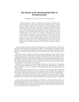
- 9. VOL. 99 NO. 6 RISK OF ENTREPRENEURSHIP 9 cumulative distribution G. We let (5) ˜Nτ = t MLtIt,τ , so (6) gv,τ = Nv,τ ˜Nτ . Our method for estimating the joint distribution is equivalent to estimating a hazard function showing the probability of exit at a given age conditional on no earlier exit, using all available data on the hazard at each age. This approach to estimating the joint distribution does not constrain it to sum to one. In our data, the sum is 0.83 . Any reasonable approach to imposing that constraint could be rationalized as the minimization of some weighted distance function. We choose the obvious one, which is to divide the distribution from (6) by the sum of all of its values. Figure ?? shows the estimated joint distribution. The left row, with literally zero exit value to the entrepreneur, dominates the probability. Most of the remaining probability goes to moderate exit values with relatively brief lifetimes. Exit values above $100 million are quite rare. Table 2 shows the joint distribution numerically, along with the marginal distributions of exit value and venture lifetime. We find 21 instances where the entrepreneur received at least $100 million and the venture lifetime was 12 months or less—of these, 9 were IPOs and the remaining 12 acquisitions. Figure 1: Joint Distribution of Venture Lifetime and Exit Value 0 05 0.06 0.07 0.08 0.09 0.10 Fraction 0 to 1 1 to 2 2 to 3 3 to 4 4 to 5 5 to 6 6 to 7 7 to 9 10+ 0.00 0.01 0.02 0.03 0.04 0.05 0 0 to 1.5 1.5 to 3 3 to 6 6 to 10 10 to 25 25 to 50 50 to 100 100 to 250 250 to 500 500+ Venture lifetime, years Exit value, millions of dollars
- 10. 10 THE AMERICAN ECONOMIC REVIEW DECEMBER 2009 The marginal distributions shown in Figure 2 and Figure 3 and tabulated in Table 2 provide useful alternative views of the joint distribution. Figure 2 shows the marginal distribution of exit value, summed across all the lifetime categories. It shows that 75 percent of all startups deliver zero exit value. Categories of low but positive exit value account for most of the rest of the outcomes. Only a tiny fraction of entrepreneurs receive more than $100 million in exit value. Figure 3 shows the conditional distribution of lifetime given exit value. Each row sums to one. Note that the two axes on the floor are reversed relative to Figure ?? to make it easier to see the shape of the distribution. This figure shows the negative correlation of lifetime and exit value. At the front, the figure shows that zero-value exits tend to have long lifetimes. At the back, it shows that high-value exits tend to have short lifetimes. The conditional distributions of the high-value exits are irregular because there are few of them, though they account for a significant fraction of the total exit value. 0.7493 0 7 0.8 0.6 0.7 0 4 0.5 Exits 0.3 0.4 Fraction of E 0 0633 0.1 0.2 0.0633 0.0340 0.0391 0.0287 0.0416 0.0211 0.0121 0.0069 0.0021 0.0018 0.0 0.1 0 0 to 3 3 to 6 6 to 12 12 to 20 20 to 50 50 to 100 100 to 200 200 to 500 500 to 1000 1000+ Figure 2: Marginal Distribution of Exit Value The fraction of entrepreneurs who received nothing in equity value from their efforts was large throughout the period covered by our data, ranging from 58 percent in 2006 through 2008 to 87 percent in 1999 through 2001. The conventional wisdom that only about half of entrepreneurs fail to receive any equity return is inconsistent with our findings. Figure 4 shows the distribution of the total exit value facing an entrepreneur, by exit- value category. Each bar shows the fraction of the total arising within the category. The category contributing the greatest fraction of value is a billion dollars or more, despite the rarity of such payoffs. Figure 5 shows the marginal distribution of venture lifetimes. The modal lifetime is between one and three years. The median is somewhat above 4 years. We do not calculate a mean lifetime, because the mean is sensitive to the extreme values, which are difficult to measure. Figure 6 shows the distribution of exit value by lifetime. More than a quarter of
- 11. VOL. 99 NO. 6 RISK OF ENTREPRENEURSHIP 11 0 3 0.3 0.4 0.4 0.5 Fraction 0 0 to 3 3 to 6 6 to 12 12 to 20 20 to 50 50 to 100 100 to 200 200 to 500 500 to 1000 1000+ 0.0 0.1 0.1 0.2 0.2 0.3 0 to 1 1 to 2 2 to 3 3 to 4 4 to 5 5 to 6 6 to 7 7 to 9 10+Venture lifetime, years Exit value, millions of dollars Figure 3: Conditional Distribution of Venture Lifetime Given Exit Value the total value arises from companies with venture lifetimes between one and two years. Not only is this range of lifetimes common, but exits that soon tend to have higher values. V. Economic Payoffs to Entrepreneurs Venture-backed companies typically have a scientist or similar expert, or a small group, who supply the original concept, contribute a small amount of capital, and find investors to supply the bulk of the capital. These entrepreneurs, together with any angels, own all of the shares in the company prior to the first round of venture funding. The entrepreneurs are specialized in ownership of the venture-stage firm. Our approach to valuation takes account of the heavy exposure of the entrepreneur to the idiosyncratic volatility of the company. We also take account of the modest salaries that entrepreneurs generally receive during the venture phase of the development of their companies and of the lifetime of the company, which affects the discounting applied to the exit value and the burden of the low salary. Our model assumes that the entrepreneurs in a company have already made all of their financial investments in their company; all further funds will come from venture investors. We believe this assumption to be generally realistic, though of course some entrepreneurs are able to continue financing their companies alongside venture investors. We portray an entrepreneur as having some savings available to finance consumption beyond what the relatively low venture salary will support. We rule out the possibility that an entrepreneur could borrow against future earnings or against the possible exit value of the company. We are quite sure this assumption is realistic. Thus the entrepreneur makes a decision
- 12. 12 THE AMERICAN ECONOMIC REVIEW DECEMBER 2009 0.283 0 25 0.30 0.195 0.225 0.20 0.25 0.170 0.15 al Value 0.10 action of Tota 0.010 0.018 0.042 0.057 0.05 Fra 0.000 0.000 0.000 0.00 0 0 to 3 3 to 6 6 to 12 12 to 20 20 to 50 50 to 100 100 to 200 200 to 500 500 to 1000 1000+ Exit value, millions of 2006 dollars Figure 4: Fractions of Total Exit Value by Exit-Value Category each year about how much to draw down savings during the year; that is, by how much consumption will exceed the venture salary. A. Analytical framework Our framework starts from a standard specification of intertemporal preferences for entre-preneurs—they order random consumption paths according to (7) E t 1 1 + r t u(ct). Here r is the entrepreneur’s rate of time preference and the rate of return on assets; u(c) is a concave period utility. We define the function U(W) as the utility from a constant path of consumption funded by wealth W: (8) U(W) = 1 + r r u r 1 + r W The multiplication by 1+r r turns flow utility into discounted lifetime utility. The quantity r 1+r W is the flow of consumption to be financed by the return on the wealth at rate r. We distinguish between wealth, Wt, which measures the entrepreneur’s total command over resources, and so incorporates the expected value of future compensation (human wealth), and assets, At, by which we mean holdings of non-human wealth as savings. At does not include the entrepreneur’s holdings of shares in the startup, which we classify
- 13. VOL. 99 NO. 6 RISK OF ENTREPRENEURSHIP 13 0.10 0.12 0.14 0.16 0.18 action 0.00 0.02 0.04 0.06 0.08 0 to 1 1 to 2 2 to 3 3 to 4 4 to 5 5 to 6 6 to 7 7 to 9 10+ Fra Venture lifetime, years Figure 5: Marginal Distribution of Venture Lifetime as human capital. For an entrepreneur in year t of a startup that has not yet exited, we define Wt(At) as the wealth-equivalent of the entrepreneur’s command over resources, counting what remains of the entrepreneur’s original non-human wealth, At, and the entrepreneur’s random future payoff from the startup, conditional on not having exited to this time. Our definition is implicit: U(Wt(At)) is the expected utility from maximizing equation (7) over consumption strategies. Now we let U(Wt(At)) be the value, in utility units, associated with an entrepreneur in a non-exited company t years past venture funding, as a function of current non- entrepreneurial assets At. We could have defined a value function Ut(At) without inter- posing the function Wt(At). Instead we let Wt(At) be the value function, which means that we need to take the concave transformation U(Wt(At)) so that the Bellman equation adds up utility, according to the principle of expected utility. The slightly roundabout approach of stating our findings in terms of the wealth-equivalent Wt(At)) makes the units meaningful, whereas the units of utility are not. Further, in our benchmark case, utility is negative, a further source of confusion. Note that W captures initial assets, ven- ture salary, venture exit value, and subsequent compensation in a post-venture position, when it is calculated at time zero for an entrepreneur. The company has a conditional probability or hazard πt of exiting at age t. At exit, it pays a random amount Xt to the entrepreneur. Upon exiting, the entrepreneur’s value function is U(W∗ (A)), where A now includes the cash exit value. The entrepreneur’s consumption is limited by assets left from the previous year—no borrowing against future
- 14. 14 THE AMERICAN ECONOMIC REVIEW DECEMBER 2009 0.15 0.20 0.25 Value 0.00 0.05 0.10 0 to 1 1 to 2 2 to 3 3 to 4 4 to 5 5 to 6 6 to 7 7 to 9 10+ Fraction of Total Exit Venture lifetime, years Figure 6: Fractions of Total Exit Value by Venture Lifetime earnings may occur. The entrepreneur’s dynamic program is (9) U(Wt(At)) = max ct<At [u(ct) + 1 1 + r (1 − πt+1)U(Wt+1((At − ct)(1 + r) + w)) + 1 1 + r πt+1 EX U(W∗ ((At − ct)(1 + r) + Xt+1))] The post-venture value function is (10) U(W∗ (A)) = 1 + r r u rA + w∗ 1 + r . Here w∗ is post-venture compensation, including employee stock options, at the non- venture continuation of this company or another company. From equations (8) and (10), we have (11) W∗ (A) = A + w∗ r . Note that this is additive in A. But when future earnings are random, the entrepreneur’s risk aversion enters the calculation of the wealth-equivalent. We represent each of the value functions U(Wt(At)) as piecewise linear with 500 knots between zero and $49 million, spaced exponentially. We calculate them by backward recursion (value function iteration). We assume power utility with constant relative risk aversion, γ. We take as our base case γ = 2, a venture salary w equal to the post-tax
- 15. VOL. 99 NO. 6 RISK OF ENTREPRENEURSHIP 15 value of $150, 000, post-venture compensation w∗ equal to the post-tax value of $300, 000, and starting assets of A0 = $1 million. A useful feature of the wealth-equivalent is that the difference between its value for an entrepreneur with given initial assets and its value for an individual who holds a non- venture position paying w∗ and with the same initial assets is the amount that the second would be willing to pay to become an entrepreneur. We call this the certainty-equivalent value of the entrepreneurial opportunity and denote it ˜A. This property follows from the additivity of the non-entrepreneurial wealth-equivalent we noted earlier. B. Results Figure 7 shows W0(A0), the wealth-equivalent for an entrepreneurial experience as of its beginning and W∗ (A0), the wealth-equivalent for a non-entrepreneur, both as functions of the common value of their initial assets, shown on the horizontal axis. The certainty- equivalent value of the venture opportunity is the vertical difference between the two curves. The non-entrepreneurial value is a straight line with unit slope—a dollar of extra initial assets becomes a dollar of wealth, because we assume that the non-venture individual faces no uncertainty. On the other hand, a dollar of extra initial assets becomes more than a dollar of equivalent wealth, because initial wealth has no uncertainty and thus dilutes the uncertainty from the venture outcome. This property is a cousin of the principle that people should treat risky outcomes as if they were worth essentially their expected values, when the outcomes are tiny in relation to their wealth. The slope of the entrepreneur’s value is more than three at low levels of assets but declines to 1.03 at assets of $20 million. 30 ollars 20 25 ionsofdo Entrepreneur 15 20 ealth,milli Non-Entrepreneur 10 valentwe 5 reerequiiv 0 0 2 4 6 8 10 12 14 16 18 20 Car Figure 7: Certainty-Equivalent Career Wealth for Entrepreneurs and Non-Entrepreneurs The figure shows that, despite the chance of making hundreds of millions of dollars in
- 16. 16 THE AMERICAN ECONOMIC REVIEW DECEMBER 2009 a startup, the economic advantage of entrepreneurship over an alternative career is not substantial. The burden of the idiosyncratic risk of a startup falls most heavily on those with low initial assets. The entrepreneur with less than a million dollars of initial assets faces a heavy burden from the risk and has a lower certainty-equivalent wealth than the non-entrepreneur. Table 3 gives the certainty-equivalent value of the entrepreneurial opportunity for 36 combinations of the three determinants: the coefficient of relative risk aversion, the com- pensation at an alternative, non-entrepreneurial job, and the entrepreneur’s assets at the beginning of entrepreneurship. The first three lines take the entrepreneur to be risk- neutral, so the values are just present values at the 5-percent annual real discount rate. In this case, the value is the same for any level of initial assets. The value is $5.8 million. The value is $5.1 million for an individual with a non-entrepreneurial opportunity to earn $600,000 per year before tax. If the non-entrepreneurial opportunity pays $2 million per year before tax, the venture opportunity has barely positive value. A typical startup probably cannot attract an established top executive from a large public corporation, even if the executive is risk-neutral, as their earnings are generally even higher than $2 million. Table A.4 in the Appendix gives estimated standard errors of the figures in Table 3. They are sufficiently small that none of our conclusions is much clouded by sampling variation. The conclusions from the table are similar if the individual is mildly risk-averse, with a coefficient of relative risk aversion of 0.9. The advantage of the entrepreneurial oppor- tunity, stated as a wealth-equivalent, is only $0.6 million for an entrepreneur with $0.1 million in assets and only $1.2 million for an entrepreneur with $5 million. These figures are negative or only slightly positive if the non-entrepreneurial opportunity pays $600,000 per year before tax. At the standard value of the coefficient of relative risk aversion, 2, the advantage of the entrepreneurial opportunity is generally small or negative—deeply negative if the non-entrepreneurial opportunity pays $2 million per year. In our base case, with non- entre-preneurial compensation of $300,000 per year before tax and $1 million in assets, the advantage of the entrepreneurial opportunity is only $0.2 million. The incentive is not impressive for larger asset holdings. With higher compensation at the non-entrepreneurial job, the advantage disappears unless the individual is quite rich. C. Implications of correlation between the number of entrepreneurs in a company and its exit value The results earlier in this section rest on the assumption that companies with more entrepreneurs have the same distribution of exit values as do other companies. We have solved the dynamic program in our base case with an alternative specification that im- plies a ratio greater than one of average exit value of companies affiliated with a single entrepreneur to the average exit value of companies affiliated with an entrepreneur with less than a 20 percent share of total entrepreneurial equity. The third column of Table 1 shows that the ratio is 1.9 within our sample of IPOs. Our alternative specification matches that ratio. The solution to the dynamic program is very similar with the alternative specification. In our base case, the value of initial savings A0 that makes the entrepreneur indifferent between entrepreneurship and the outside salary opportunity is $188,949 , while the indifference point for the alternative is $184,352 .
- 17. VOL. 99 NO. 6 RISK OF ENTREPRENEURSHIP 17 VI. Entrepreneurs in Aging Companies Our discussion so far has focused on the risk-adjusted payoff to a potential entrepreneur at the decision point when venture funding first becomes available. In this section, we consider the same issue at later decision points, as the startup ages. Our discussion is conditional on the company not having exited. The dynamic program of equation (9) assigns a value Wt(At) to the entrepreneur’s position in each year t that the company has not exited. Under our assumptions, the path is the same for all companies. The entrepreneur’s value falls as the company ages for two reasons. First, the entrepreneur generally consumes out of assets, so assets decline. Second, early exits are the most valuable exits, so aging another year means that the remaining potential exit values are not as valuable. Figure 8 shows the path of Wt(At). It declines from $5.1 million at the outset to $4.3 million at age 10, conditional on no exit. From that point, the value rises, because the distribution of exit values becomes more favorable, though not as favorable as for young startups. The figure also shows the individual’s value of a non-entrepreneurial job, W∗ (At). It declines as well, but only for the first reason, the draw-down of assets to finance consumption in excess of the low startup salary. 4.4 4.6 4.8 5.0 5.2 s of dollars Wt(At) W*(At) 3.4 3.6 3.8 4.0 4.2 1 2 3 4 5 6 7 8 9 10 11 12 13 14 15 16 17 Million Year Figure 8: Entrepreneurial Value and Non-Entrepreneurial Value Prior to Exit Figure 9 shows the paths of assets and consumption as a company ages. For the first decade, assets decline because consumption exceeds the modest startup salary and the entrepreneur has no other source of current cash, pending a favorable exit. During this period consumption declines, because, as an exit fails to occur during the early
- 18. 18 THE AMERICAN ECONOMIC REVIEW DECEMBER 2009 years, the entrepreneur learns that risk-adjusted well being, as measured by Wt(At), has declined. Eventually assets fall to the point of consumption. From this point until exit, the entrepreneur lives on the salary and maintains assets only as a way to spread consumption between paychecks (we assume, for simplicity, that the entrepreneur receives the salary at the end of each year and we measure assets at the beginning of the year). The line labeled c(Wt) shows the level of consumption that a consumer without a cash-flow constraint would choose, given lifetime prospects as measured by Wt. Consumption starts out only slightly below this level, but as the entrepreneur depletes assets, consumption falls toward the cash-flow limit. In the event that the startup ages into its second decade, the cash-flow constraint keeps consumption far below its unconstrained level. 0.6 0.8 1.0 1.2 s of dollars Assets 0.0 0.2 0.4 1 2 3 4 5 6 7 8 9 10 11 12 13 14 15 16 17 Millions Year c(Wt) Consumption Figure 9: Consumption and Assets prior to Exit VII. Robustness and Related Results Table 4 shows certainty-equivalent values for a variety of alternative specifications. The first line repeats the base case from Table 3. The second line limits the companies included in the calculations to those in information technology. In all but the top initial wealth category, the values are slightly lower for these companies than for venture-backed companies in general. For the less risk-averse entrepreneurs in the top wealth category, the value is higher, reflecting disproportionate role of IT in the most successful startups, such as Google. The third line limits the companies to those in biotech. The certainty- equivalent value of a biotech startup is higher in every wealth category. The fourth and fifth lines of Table 4 break the sample by the date of first venture funding. The basic conclusions of the paper apply equally to companies launched in 1995
- 19. VOL. 99 NO. 6 RISK OF ENTREPRENEURSHIP 19 and earlier and to those launched after 1995. Line 6 of the table explores the sensitivity of our calculations to our procedure for imputing the dilution of the entrepreneur’s share in a round of venture funding when the dilution is not reported directly. We add one percent to the fitted value from the logit regression that imputes the share of the company in all such rounds sold to that round’s group of venture investors. The extra dilution depresses the entrepreneur’s certainty- equivalent value, but the change does not affect any of our conclusions. Line 7 calculates the effect of the provisions of the standard venture contract that shift ownership to the investors at the expense of the entrepreneurs and other common shareholders in the case of a down round. In such a round, the share price is below the price of an earlier round. The increase is tiny—the great bulk of payoffs to entrepreneurs come from IPOs and higher value acquisitions and companies enjoying these favorable outcomes rarely experience down rounds. Line 8 changes the cutoff for diagnosing a company that has reached the point of little likelihood of any equity payoff to the entrepreneur. The cutoff is five years in the base case; we change it to four years here. The result is to include somewhat more recent companies and to lower the certainty-equivalents slightly, but not in a way that changes any of our conclusions. Line 9 calculates the effect of the preference provisions of the standard venture contract that provide extra cash to the investors at the expense of the entrepreneurs and other common shareholders. The increase is noticeable—these provisions raise entrepreneurial risk and lower expected returns because they increase entrepreneurs’ leverage. We be- lieve we have correctly incorporated the preferences in our calculations. This calculation illustrates the importance of the preferences, not a potential error in our work. Lines 10 and 11 show the results of two similar alterations of our calculations. One is to boost the initial entrepreneurial ownership by one percent at the expense of the angels and other pre-venture investors. The other is to boost the ownership granted the entrepreneurs by the incentive provisions of the venture contract. Both result in small increase in the certainty-equivalent values. Line 12 shows a reverse calculation, where the share granted the non-entrepreneur employees, such as a CEO hired to replace an entrepreneur, dilutes the entrepreneur. This alteration results in a small decline in certainty-equivalent value. Line 13 probes the sensitivity to the parameter that controls the relation between the success of the company and the entrepreneur’s incentive ownership. We chose this pa- rameter based on our own judgment, in view of the absence of any systematic information about the incentive provisions in actual venture contracts. The calculation shows that our conclusions are not sensitive to the value of the parameter. Most entrepreneurial exit value comes from great success—IPOs or favorable acquisitions—where presumably the entrepreneurs get the maximum incentive ownership. Line 14 drops the largest single entrepreneurial payoff, Google. It has no visible effect on the results. At a coefficient of relative risk aversion of 2, the prospective entrepreneur puts very little additional weight on a billion-dollar payoff compared to a hundred-million one. Line 15 makes the unrealistic assumption that entrepreneurs receive cash for their shares at the IPO price, at the time of the IPO, in place of our assumption that they cannot sell shares in the IPO or in the public market for 6 months after the IPO. The average return earned over that 6-month period is over 50 percent. Nonetheless, the certainty-equivalent value of the entrepreneur is higher if ownership is liquidated at the IPO and the entrepreneur foregoes the expected 50-percent return in favor of the benefit of diversification. To put it differently, the entrepreneur would be better off by selling at the low IPO price rather than taking a chance on the post-IPO appreciation (the “pop”).
- 20. 20 THE AMERICAN ECONOMIC REVIEW DECEMBER 2009 Typically, the IPO price drives the entrepreneur’s marginal utility down to close to zero. A few companies lose all or most of their value in the 6 months after their IPOs. It is worthwhile for the entrepreneur to cut off this chance by selling in the IPO. Thus, the lockup period in the typical venture-capital contract is another feature that imposes substantial idiosyncratic risk on the entrepreneur. VIII. Sorting between Entrepreneurship and Employment The coexistence of the entrepreneurial and employment contract forms for bringing new high-tech products to market presumably reflects heterogeneity on both sides of the market. Where powerful incentives are less important, large organizations will domi- nate because they can insure their workers. In this section, we examine sorting among individuals by deriving the crossover point for the choice of an individual between en- trepreneurship and employment. We divide the three-dimensional space defined by risk aversion, alternative employment compensation, and initial assets into two subspaces, one where the individual prefers to be an entrepreneur and the complement where the individual prefers to be an employee. Figure 10 shows the surface separating the two subspaces, as a set of lines in the risk aversion-starting assets plane. Each line shows the dividing line in the plane correspond- ing to a different value of the compensation available at alternative employment. The line at the lower right describes people who are indifferent between employment and entrepreneurship when employment pays a safe $300,000 per year or more, before tax. Those below and to the right of the line definitely prefer employment. The next line up and to the left shows indifference when the outside salary is $500,000. The region between the two lines describes people who are more inclined to entrepreneurship than those in the slender wedge at the bottom, because they have less risk aversion or more savings, or both. Similarly, the next line up and to the left describes indifference when outside compensation is $700,000. Those choosing entrepreneurship despite high outside earnings have quite low risk aversion or high savings. Other characteristics may affect the sorting of engineers and scientists into entrepreneur- ship and employment. Those with a preference for working in an organization they help manage or a distaste for an employment hierarchy will choose entrepreneurship even if they are located clockwise of the relevant line in Figure 10. Another possibility is that entrepreneurship attracts individuals who overestimate the likely payoffs from their ideas. IX. Discounting We stress that the parameter r in our analysis is the rate of time preference and also the return earned on the entrepreneur’s savings. It is not the financial discount rate or cost of funds of the startup company. Financial discounting is implicit in the dynamic program. We can illustrate the high implicit discount by a simple thought experiment. Suppose that an entrepreneur learned in year t that an exit would occur in the following year, and the entrepreneur owned a security that paid off Xt+1 in year t+1, where is a small amount. Any individual trades off small values in one period against another period at the marginal rate of substitution. Thus the value the entrepreneur would ascribe to the security would be (12) EX u (ct+1) (1 + r)u (ct) Xt+1
- 21. VOL. 99 NO. 6 RISK OF ENTREPRENEURSHIP 21 5 6 7 8 9 10 lionsofDollars w* ≥ $700,000 0 1 2 3 4 5 0.50 0.70 0.90 1.10 1.30 1.50 1.70 1.90 2.10 2.30 2.50 2.70 2.90 InitialAssets,Mill Coefficient of Relative Risk Aversion w* ≥ $500,000 w* ≥ $300,000 Figure 10: Sorting of Individuals into Entrepreneurship and Employment The discount factor Dt is the ratio of this value to the expected value, (13) Dt = EX u (ct+1) (1+r)u (ct) Xt+1 EX Xt+1 In our base case, with coefficient of relative risk aversion of two, the discount factor Dt varies from 0.01 to 0.04 over the age of the company. Thus a claim that had an expected payoff of one dollar next year, in proportion to the distribution of the exit value next year, would be worth only $0.01 to $0.04 this year. Conceptually, the discount breaks down into a pure time element and an element relating to the fact that the amount of the exit value will become known next year. The pure time discount is just the 5 percent in 1 1+r . All the rest of the discount comes from the uncertainty in the exit value. The reason that the entrepreneur puts such a low value on the payoff Xt+1 is that it delivers almost all its value in circumstances where the entrepreneur is rich and has low marginal utility. Notice that D = 1 1.05 for a risk-neutral entrepreneur with constant marginal utility. X. Serial Entrepreneurship Paul Gompers, Anna Kovner, Josh Lerner and David Scharfstein 2008 report that about 12 percent of venture-backed entrepreneurs have served in that role in an earlier venture-backed startup. Our dynamic program, equation (9), does not consider that possibility. We could alter the program to include the 12 percent likelihood of future entrepreneurship, though this alteration would come at a considerable complication in calculating the value functions, because the same function would appear after the exit in the future and at time zero. The effect would be a slight increase in the value of
- 22. 22 THE AMERICAN ECONOMIC REVIEW DECEMBER 2009 entrepreneurship relative to employment. None of our conclusions would be significantly affected, because the probability of repeating as an entrepreneur is relatively small. Our results have an interesting implication for serial entrepreneurship. Figure 10 shows that the choice between entrepreneurship and employment is sensitive to assets. A suc- cessful exit will give an entrepreneur a substantial level of assets, far up the vertical axis in the figure. Hence further entrepreneurship becomes far more attractive relative to employment after a success. Wealth from a successful earlier exit relieves the burden of the idiosyncratic risk of a second startup. XI. Concluding Remarks The contract between venture capital and entrepreneurs does essentially nothing to alleviate their financial extreme specialization in their own companies. Given the nature of the gamble revealed in Figure 2, entrepreneurs would benefit by selling some of the value that they would receive in the best outcome on the right, when they would be seriously rich, in exchange for more wealth in the most likely of zero exit value, on the left. It would be hard to find a more serious violation of the Borch-Arrow optimality condition—equality of marginal utility in all states of the world—than in the case of entrepreneurs. A diversified investor would be happy to trade this off at a reasonable price, given that most of the risk is idiosyncratic and diversifiable. But venture capitalists will not do this—they don’t buy out startups at the early stages and they don’t let entrepreneurs pay themselves generous salaries. They use the exit value as an incentive for the entrepreneurs to perform their jobs. Moral hazard and adverse selection bar the provision of any type of insurance to entrepreneurs—they must bear the huge risk shown in Figure 2. The venture capital institutions of the United States convert ideas into functioning businesses. We show that the process contains an important bottleneck—for good reasons based mainly on moral hazard, the venture contract cannot insure entrepreneurs against the huge idiosyncratic risk of a startup. Risk-adjusted payoffs to the entrepreneurs of startups are remarkably small. Although our results are based entirely on the venture process, we believe that no other arrangement is much better at solving the problem of getting smart people to commercialize their good ideas.
- 23. VOL. 99 NO. 6 RISK OF ENTREPRENEURSHIP 23 Table 2: Joint Distribution of Venture Lifetime and Exit Value, Percent Probability by Cell 0 to 1 1 to 2 2 to 3 3 to 4 4 to 5 0 6.37 12.85 11.69 10.44 8.58 0 to 3 0.189 0.681 0.733 0.829 0.816 3 to 6 0.131 0.411 0.402 0.472 0.427 6 to 12 0.180 0.489 0.519 0.573 0.477 12 to 20 0.132 0.406 0.408 0.431 0.366 20 to 50 0.238 0.642 0.624 0.607 0.554 50 to 100 0.131 0.414 0.363 0.310 0.254 100 to 200 0.061 0.267 0.231 0.226 0.143 200 to 500 0.036 0.159 0.141 0.159 0.082 500 to 1000 0.0058 0.0559 0.0341 0.0848 0.01098 1000+ 0.00141 0.04510 0.03115 0.07951 0.00975 All 7.47 16.42 15.17 14.21 11.72 Exit value (millions of dollars) Venture Lifetime, years 5 to 6 6 to 7 7 to 9 10+ All 0 6.38 4.99 6.63 7.01 49.9 0 to 3 0.778 0.621 0.854 0.834 3.25 3 to 6 0.426 0.331 0.416 0.381 1.84 6 to 12 0.457 0.352 0.471 0.391 2.24 12 to 20 0.312 0.232 0.318 0.262 1.74 20 to 50 0.433 0.371 0.397 0.294 2.66 50 to 100 0.190 0.167 0.168 0.112 1.47 100 to 200 0.084 0.059 0.083 0.061 0.93 200 to 500 0.044 0.016 0.023 0.032 0.575 500 to 1000 0.00513 0.00389 0.00203 0.00246 0.192 1000+ 0.01593 0.00000 0.00000 0.00000 0.167 All 9.12 7.14 9.36 9.38 65 Exit value (millions of dollars) Venture Lifetime, years
- 24. 24 THE AMERICAN ECONOMIC REVIEW DECEMBER 2009 Table 3: Certainty-Equivalent Value of the Venture Opportunity 0.1 1 5 20 0 300 5.8 5.8 5.8 5.8 0 600 5.1 5.1 5.1 5.1 0 2,000 2.3 2.3 2.3 2.3 0.9 300 0.6 0.9 1.2 1.8 0.9 600 -0.2 0.3 0.7 1.2 0.9 2,000 -5.8 -4.0 -2.1 -1.6 2 300 -0.1 0.2 0.5 1.1 2 600 -1.8 -0.6 -0.1 0.5 2 2,000 -13.9 -8.9 -3.7 -2.2 Coefficient of relative risk aversion, γ Pretax compensation at non- entrepreneurial job, thousands of dollars per year Certainty-equivalent of entrepreurial opportunity, millions of dollars Assets at beginning, millions of dollars
- 25. VOL. 99 NO. 6 RISK OF ENTREPRENEURSHIP 25 Table 4: Alternative Specifications and Robustness Checks 0.1 1 5 20 1 Base case from 7th line of Table 3 15,209 -0.10 0.22 0.48 1.06 2 Information technology companies only 7,318 -0.08 0.25 0.53 1.15 3 Biotech companies only 3,818 0.07 0.49 0.93 1.95 4 Companies first funded from 1987 through 1995 5,019 -0.12 0.27 0.58 1.19 5 Companies first funded after 1995 10,190 -0.09 0.19 0.43 1.00 6 Add 1 percent to imputed venture ownership share for rounds where company value was not reported 15,209 -0.11 0.21 0.47 1.05 7 Eliminate deduction from entrepreneurs' ownership for down rounds 15,210 -0.10 0.23 0.50 1.10 8 Change 5-year cutoff for imputed exit to 4 years 15,760 -0.12 0.19 0.45 1.01 9 Remove deduction from entrepreneurs' exit value for preferences 15,210 -0.02 0.33 0.64 1.30 10 Increase initial entrepreneurs' share by 1 percent 15,209 -0.10 0.22 0.49 1.07 11 Increase entrepreneurs' extra potential incentive ownership by 1 percent 15,209 -0.10 0.22 0.49 1.08 12 Increase employees' extra potential incentive ownership by 1 percent 15,209 -0.10 0.21 0.48 1.06 13 Reduce the gross return ratio where full incentive ownership is granted (ψ) from 8 to 7 15,209 -0.10 0.22 0.49 1.07 14 Remove Google 15,208 -0.10 0.22 0.48 1.06 15 Entrepreneurs receive cash at IPO rather than 6 months later 15,210 -0.06 0.26 0.54 1.12 Case Certainty-equivalent of entrepreurial opportunity, millions of dollars Assets at beginning, millions of dollarsNumber of exits
- 26. 26 THE AMERICAN ECONOMIC REVIEW DECEMBER 2009 REFERENCES Admati, Anat R., and Paul Pfleiderer. 1994. “Robust Financial Contracting and the Role of Venture Capitalists.” Journal of Finance, 49(2): 371–402. Bagley, Constance E., and Craig E. Dauchy. 2003. The Entrepreneur’s Guide to Business Law. West Legal Studies in Business. Casamatta, Catherine. 2003. “Financing and Advising: Optimal Financial Contracts with Venture Capitalists.” Journal of Finance, 58(5): 2059–2085. Gompers, Paul, Anna Kovner, Josh Lerner, and David Scharfstein. 2008. “Per- formance Persistence in Entrepreneurship.” Harvard Business School Working Paper 09-028. Hall, Robert E., and Susan E. Woodward. 2007. “The Incentives to Start New Companies: Evidence from Venture Capital.” Hoover Inistitution, Stanford University, stanford.edu/∼rehall. Heaton, John, and Deborah Lucas. 2004. “Capital Structure, Hurdle Rates, and Portfolio Choice—Interactions in an Entrepreneurial Firm.” University of Chicago and Northwestern University. Kaplan, Steven N., and Per Stromberg. 2003. “Financial Contracting Theory Meets the Real World: An Empirical Analysis of Venture Capital Contracts.” Review of Eco- nomic Studies, 70: 281–315. Repullo, Rafael, and Javier Suarez. 2004. “Venture Capital Finance: A Security Design Approach.” Review of Finance, 8: 75–108. Schmidt, Klaus M. 2003. “Convertible Securities and Venture Capital Finance.” Jour- nal of Finance, 58(3): 1139–1166. Wilmerding, Alex. 2003. Deal Terms: The Finer Points of Venture Capital Deal Struc- tures, Valuations, Term Sheets, Stock Options, and Getting Deals Done. Aspatore.
- 27. VOL. 99 NO. 6 RISK OF ENTREPRENEURSHIP 27 Appendix Data Investment Rounds We use the standard and convenient vocabulary for describing the evolution of the value of a venture-backed company. When a round of funding occurs, the venture syndicate negotiates a price per share with the entrepreneurs or other management of the company. This price, multiplied by the number of shares outstanding before the new funding, is called the pre-money value of the company. The sum of the pre-money value and the amount newly invested is the post-money value. The two values together fully describe the financial evolution of the company, without reference to the share prices or the number of shares. The return ratio earned by shareholders is the ratio of the new pre-money value to the previous post-money value. The pre-money value is adjusted by GP fees and preferences in the case of an exit event. Venture investors make a series of investments, f1 through fN , in months t1 through tN . Immediately before a round, the pre-money value of the firm is vi. At time τ, either the company undergoes an initial public offering, is acquired, or ceases operations, with an exit cash payoff to the investors of x. We let si,j be the ownership share of the company attributable to the investment in round i as of round j. The initial ownership share is (14) si,i = fi fi + vi . Later rounds dilute the share according to the recursion, (15) si,j = si,j−1vj fj + vj . The exit value of round i investors is xi = si,N+1x. Adjustment of Ownership Shares in Down Rounds A down round occurs when the share price or pre-money value in one round is below the previous round. Most agreements between venture investors and entrepreneurs call for the issuance of additional shares to investors in earlier rounds when the share price in a new round falls short of the price in the previous round—what is called a “down round.” The adjustment is set forth in anti-dilution provisions in the agreements. Steven N. Kaplan and Per Stromberg 2003 find that about a quarter of the contracts have full- ratchet language, meaning that the entrepreneurs absorb enough of the decline in value to leave the value of venture’s ownership at the same level as in the previous round. The other three quarters of contracts have a more moderate provision called weighted-average adjustment. Both types of anti-dilution adjustments are modifications of equation (15) to shift ownership shares toward venture investors who paid more than the current price for their shares, where the price paid is measured on a post-conversion basis. We calculate updated ownership shares for down rounds using both types of adjustment and take the weighted average, using the figures from Kaplan and Stromberg 2003.
- 28. 28 THE AMERICAN ECONOMIC REVIEW DECEMBER 2009 Down-round anti-dilution provisions shift venture ownership upward and non-venture (entrepreneurs, angels, and employees) downward by an average of 4.8 percentage points. These provisions reduce the reward to entrepreneurs disproportionately in the less favor- able outcomes. The weighted-average anti-dilution provision is the most common form of adjustment. To explain this provision, we let j be the number of the current round and let i range over the earlier rounds. We let ni,j be the number of shares effectively held by round i investors as of round j. “Effectively” means the number of common shares that would result from the investors exercising their conversion rights. Anti-dilution provisions take effect by lowering the conversion price, pi,j, and increasing the number of shares, ni,j = fi/pi,j, the investors receive upon conversion. We let Ni,j be the total number of shares outstanding at the conclusion of round j. To identify the investors eligible for the anti-dilution adjustment without knowing actual share counts and share prices, we proceed as follows: The conversion price per ownership share point for earlier investors as of the last round is fi/si,j−1. The price per ownership point (measured as of the previous round) paid by the new round is the pre-money value vj. Thus the eligible rounds are those with fi/si,j−1 > vj. We let Aj designate the set of these rounds and ∼ Aj the set of rounds not subject to adjustment, including the common shares. The weighted-average provision specifies adjustment factors for the eligible earlier in- vestors in the case of a down round: (16) ai,j = Nj−1 + nj,j Nj−1 + pj,j pi,j−1 nj,j . The numerator is the number of shares after round j if the existing shareholders did not receive any new shares. The denominator is the number of shares if the new round had to pay the higher price paid by an investor in round i. The new conversion price is the old price divided by the adjustment factor. The quantity pj,jnj,j is fj, the amount invested in the new round. The earlier conver- sion price pi,j−1 is fi/ni,j−1. Thus (17) ai,j = Nj−1 + nj,j Nj−1 + fj fi ni,j−1 . To reduce the complexity of what follows, we write (18) bi,j = 1 Nj−1 + fj fi ni,j−1 , so the adjustment factor is (19) ai,j = bi,j(Nj−1 + nj,j). The total number of shares of the earlier investors, after adjustment for those who paid
- 29. VOL. 99 NO. 6 RISK OF ENTREPRENEURSHIP 29 more than the current price, is ˜Nj = i∈Aj bi,j(Nj−1 + nj,j)ni,j−1 + i∈∼Aj ni,j−1 = Bj(Nj−1 + nj,j) + ¯Nj.(20) The ownership share of the new round is sj,j = fj vj + fj = nj,j ˜Nj = nj,j Bj(Nj−1 + nj,j) + ¯Nj + nj,j .(21) This can be written as a linear equation in the unknown nj,j. We solve for nj,j, multiply by the expression in equation (17), and use the resulting share counts to form the new values of the ownership shares si,j. By enlarging the ownership shares for the investors who paid more than the current share price, the provision reduces the shares of the entrepreneurs and other earlier investors even more than the normal dilution from a new round. The calculations described above are homogeneous in the numbers of shares, so we can normalize the total number of shares from the previous round at one. After this normalization, ni,j−1 = si,j−1. The effect of the calculations, including forming the new shares si,j, is to modify equation (15) to include the rearrangement of equity interests among the existing shareholders that occurs in a down round. The description of the weighted-average updating in a down round given in this ap- pendix is rather more complicated than in standard references on venture contract terms, such as Bagley and Dauchy 2003. Those descriptions assume the availability of data on share holdings and conversion prices. Our approach is tailored to our data, which require us to infer these numbers from data on pre- and post-money value. In the case of the full-ratchet anti-dilution adjustment, the rearrangement of ownership shares can be expressed in the same framework. Those investors who paid more than the current price for their shares in an earlier round receive a proportional increase in ownership (decrease in conversion price) equal to the ratio of the earlier price to the current price. If an earlier round, i, had a higher price, its number of shares becomes fi/pj,j. As before, the current price is pj,j = fj/nj,j. Thus the number of adjusted shares brought into the current round is (22) i∈Aj fi fj nj,j + i∈∼Aj ni,j−1. Again, we can solve the equation for the ownership share of the new round, (23) sj,j = nj,j nj,j i∈Aj fi fj + i∈∼Aj ni,j−1 + nj,j , for the new ownership nj,j, and then calculate the ownership shares of the earlier investors and entrepreneurs. As before, the total number of shares owned as of the previous round
- 30. 30 THE AMERICAN ECONOMIC REVIEW DECEMBER 2009 can be normalized at one, so the procedure developed here is a recursion that describes the rearrangement in ownership shares that occurs in a down round because of the anti- dilution provision benefiting earlier venture investors. Sources We use a database compiled by Sand Hill Econometrics on venture investments in startups and on the fates of venture-backed companies. The data are drawn from a variety of sources, including several commercial data vendors. The vendors concentrate on reporting funding and valuations for venture investments and are less likely to report exit events, especially shutdowns and acquisitions at low values. Sand Hill Econometrics has used a wide range of sources to augment coverage of these adverse termination events. One important source of valuation data is S-1 statements filed by venture-backed com- panies when they go public. These statements often give a funding history for the com- pany. Because an IPO is a favorable event, the back-filling of round values from S-1s is a source of return-based selection in the data. Table A.1 describes the data. Our general database reports 62,609 funding rounds for 22,004 companies. Among the exit values used in the analysis, 2,015 are IPOs, 5,625 are acquisitions, and 3,352 are confirmed zero-value exits. For an additional 4,220 companies, we infer zero-value exits from the observation that the company neither exited nor raised funds in the last five years of our sample. We assign an exit date to these companies by drawing from the distribution of time from last funding to exit for the companies with known failure dates. Table A.1: Counts in Database Number Companies 22,004 Inferred to be active private companies as of December 2008 6,792 Exits 15,212 IPO 2,015 Acquisition 5,625 Confirmed to have ceased operations with no value 3,352 Imputed exit with zero value for lack of funding for 5 years 4,220 Funding rounds 62,609 With ownership share from new investment revealed 16,637 With imputation of ownership share 45,972 Second look rounds (all with value revealed) 1,292 With value not revealed in main data 762 Of the 62,609 funding rounds included in the analysis, we can infer the venture share directly from the reported value in 16,637 of the rounds. In the remaining 45,972 rounds, we impute the venture share of ownership as described below. For this purpose, we use the second-look database of 1,292 funding rounds where the values (and thus venture shares) are reported for companies with missing valuations in the general database. That sub-sample contains 762 rounds.
- 31. VOL. 99 NO. 6 RISK OF ENTREPRENEURSHIP 31 Preferences The standard financial contract gives venture convertible preferred equity in a company— see Kaplan and Stromberg 2003, Table 1. In about half of these cases, venture receives both its original investment and its common-stock value, sometimes with an upper limit on the common-stock value for payment of the original investment. The second form of claim is called participating preferred stock. We do not observe the preference terms for each of the rounds of investment in our database. Further, we observe unfavorable outcomes—those in the range where the pref- erences would matter—after negotiations that altered the preferences may have occurred among the disappointed claimants on a company. We understand that venture investors sometimes bargain away their preferences and become common shareholders in order to induce the entrepreneurs to agree to a disappointing exit plan. Wilmerding 2003 writes, in connection with a low potential exit value, “. . . at those levels, where management will not receive much from a sale, the preferred shareholders will likely be forced to give up some of their return to make the deal work” (p. 52). Our data do not reveal if the cash from a low-value exit is distributed according to the original contracts or whether the parties have bargained to a jointly superior outcome once the bad news arrived. The reason that a jointly superior bargain is available is that adverse events leave the entrepreneurs, holding only common stock, with option positions that are far out of the money because of the preferences. In this situation, the entrepreneurs have little incentive to perform the functions needed to recover limited value from a disappointing outcome. They will prefer to continue rolling the dice unless a new deal can be struck that better aligns incentives. In some cases, one round of preferred stock has priority over another, but we lack information on priorities, so we assume that all rounds of preferred shares have equal priority and divide the available cash in proportion to the amount invested. Kaplan and Stromberg 2003, Table 2, report that 71 percent of venture contracts grant preferences in excess of the amount invested, often in the form of a cumulative dividend, which averages 8 percent per year. We take the preference to be 125 percent of the amount invested, corresponding to about 3 years of the dividend. For non-participating preferred shares, the cash payout is (24) max (min (¯sX, ¯sP), sX)) , where ¯s is the share of a given venture round among all venture (preferred) shareholders and s is the share of the round among all shareholders, X is the exit value of the company, and P is the preference amount for the round. For participating shares, the payout is (25) min (¯sX, ¯sP + s(X − P)) . Additional ownership for entrepreneurs and employees The contract between venture investors and entrepreneurs often includes provisions for additional ownership based on company performance. The entrepreneurs vest in the shares upon reaching milestones in the contract. In addition, non-founder employees vest in stock options based on longevity and other factors. Kaplan and Stromberg 2003, Table 2, report on both elements of vesting in terms of ownership shares if no vesting occurs and if all vesting occurs. The average founders’ share rises from 24.3 percent to 31.1 percent upon full vesting and the average share of non-founder and employee ownership rises from 20.2 percent to 22.2 percent.
- 32. 32 THE AMERICAN ECONOMIC REVIEW DECEMBER 2009 We interpret the initial 20.2 percent as the share of non-entrepreneur, non-venture investors—angels and friends of the family. We interpret the initial non-venture share observed in our data as the sum of the entrepreneurs’ share and the 20.2 percent. We interpret the incremental 2.0 percent as the ownership of non-founder employees upon a successful exit such as an IPO. We interpret the incremental 6.8 percent of entrepreneur ownership in the same way. We construct an index of success, with respect to vesting, as (26) z = min 1, X ψF , where X is the gross value to all existing shareholders at exit and F is the sum of all rounds of venture investing. The parameter ψ is interpreted as the ratio where all possible vesting occurs. We take ψ = 8. We boost the entrepreneur and non-venture investor share by 0.068z and impute a share to non-founder employees of 0.02z. Imputing missing venture ownership shares In our data, the amounts invested by venture are reported quite fully. As Table A.1 shows, however, the valuation of the company at the time of the investment is often not re- ported. We impute the missing data on the form of the ownership share acquired through the new investment. The share implies pre- and post-money values of the company at the time of the investment. We impute missing data for the venture shares by combining a standard missing-data approach with a unique body of data that provides a full solution to the problem of selection bias that plagues the imputation of missing data in most applications. Our second-look database gives full information about valuations obtained from an- other source for more than a thousand of the financing rounds in the general data. We make the imputations of venture share from the second-look database. Here we know about missing data, from the perspective of the large body of data, and about true shares, from the fully reported data. Thus we can make a direct attack on the selection problem described above. We fit an equation to the actual shares in the second-look data for the companies with missing valuations in the general database. The second-look database contains data on 2.0 percent of the funding rounds in our main database. It is reasonably representative of the main database. We measure repre- sentativeness as the ratio of funding rounds in a given category to the expected number if the second-look data were perfectly representative and thus contained 2.0 percent of the number of rounds in that category in the main database. The second-look data were collected in 2006 and do not contain any rounds since then; they also lack rounds from before 1993. The representativeness ratio is 96 percent for 1993 to 1995, 117 percent for 1996 to 1998, 155 percent for 1999 to 2001, and 149 percent for 2002 to 2004. Among major sectors, the ratio is 59 percent for information technology, 104 percent for telecom- munications, 162 percent for biotechnology, and 146 percent for retail. The ratio is 150 percent for companies that eventually went public. For rounds reported in the second- look data, the fraction reporting value in the main data was 31 percent, compared to 24 percent for all rounds in the main data. The company values reported in the second-look data (which we regard as virtually certain to be correct in the sense of being the values actually calculated by the venture funds) are generally identical to or close to the values reported in the main database. About 60 percent of the 402 rounds present in the second-look data for which values are also reported in the main data have exactly the same value in both sources. About 90
- 33. VOL. 99 NO. 6 RISK OF ENTREPRENEURSHIP 33 percent of the overlap values in the main database are within 15 percent of the second-look values. The maximum discrepancy is 41 percent. The venture share, s, needs to be tracked through the various rounds of financing as later rounds dilute the ownership of earlier rounds. The calculations require the most recent share, (27) si,i = fi fi + vi because the recursion in equation (15) can be written: (28) si,j = si,j−1(1 − si,i). We use the nonlinear logit regression specification (29) si,i = 1 1 − exp(−Xiδ) , where Xi is a vector of variables observed even when vi is missing and δ is the corre- sponding vector of parameters. As predictive variables, we use: • Number of this round • Amount raised in this round • Cumulative increase in the Wilshire index over the 2 years preceding this round Our specification has a complete set of interactions by round number, except that we fit the same coefficients for rounds 5 and higher. Table A.2 shows the results of this regression. The selection bias for the main data appears to be downward: The average value for rounds reported in both the main data and the second-look data is $22 million less than the average value reported in the second-look data for rounds in the main data where value was not reported. The difference is statistically unambiguous, with a standard error of $7 million. Joint Distribution with Positive Dependence of the Entrepreneur’s Exit Value and Share of That Value We define the latent random variable z related to total entrepreneurial exit value V by (30) z = ρV + u. Here u is a random variable distributed uniformly on the unit interval. The parameter ρ controls the strength of the dependence. The support of z is [ρV , ρV + 1], where [V , V ] is the range of values of V in the database. The marginal cdf of z is (31) Prob[z ≤ Z] = V Prob[z ≤ Z|V ]Prob[V ],
- 34. 34 THE AMERICAN ECONOMIC REVIEW DECEMBER 2009 Table A.2: Coefficients for Logit Specification for Venture Share of Ownership in a Funding Round Round Constant Amount raised Stock market 1 0.141 0.004 -0.450 (0.306) (0.004) (0.228) 2 -0.094 0.003 -0.656 (0.247) (0.003) (0.201) 3 0.017 0.003 -0.948 (0.232) (0.002) (0.210) 4 0.046 0.010 -1.192 (0.297) (0.004) (0.250) 5 or higher 0.057 0.014 -1.276 (0.219) (0.003) (0.198) Standard error of the regression: 0.160 where the summation is over all the values of V in the database. Prob[V ] is the reciprocal of the number of exit values V in the database. The conditional probability is Prob[z ≤ Z|V ] = Prob[u ≤ Z − ρV ] = 0 if Z − ρV ≤ 0(32) = Z − ρV if 0 ≤ Z − ρV ≤ 1 = 1 if Z − ρV ≥ 1. We evaluate the conditional probability at 1000 values of Z, using all of the values of V in the database. We then find the cutoff values of z, Zi, corresponding to the distribution of the entrepreneur’s share among the 6 categories. Thus, (33) Prob[s ∈ Si] = Prob[z ∈ [Zi−1, Zi]]. Here Si is the range of values of the entrepreneur’s share shown in the first column of text Table 1. When solving the consumer dynamic program, (9), we form the expectation over the entrepreneur’s exit value, X = sV , by summing over the V s in a given age group and the conditional distribution of the share, s, in the six categories, each with probability (34) Probs = ¯si = Prob[z ≤ Zi|V ] − Prob[z ≤ Zi−1|V ], where equation (32) give the conditional probability. The values ¯si are the means of the share within each category, shown in the right-most column of text Table 1.
- 35. VOL. 99 NO. 6 RISK OF ENTREPRENEURSHIP 35 We calculated the expected company exit values given the entrepreneur’s share category as follows. The probability that a given company exit value V corresponds to entrepreneur share category i as defined in text Table 1 is (35) min(1, Zi − ρV ) − max(0, Zi−1 − ρV ). We calculated E (V |i) as the sum of the V s in the sample weighted by these probabilities. We found that ρ = 0.011 equated E (V |i = 6)/ E (V |i = 1) to its value in the IPO sample of 1.9. Table A.3 shows the joint distribution of entrepreneurial exit value and venture life- time corresponding to text Table 2, but with the alternative assumption of correlation between total entrepreneurial exit value and an entrepreneur’s share. We calculate the distribution by using the conditional probabilities in (35) in place of hi in text (3). Note that the marginal distributions of the entrepreneur’s exit value are slightly different in Table A.3 from text Table 2, because we do the calculation prior to renormalizing the joint distribution. Bootstrap Standard Errors The estimates in Table 3 have sampling variation from two sources: (1) estimation of the coefficients of the equation for imputing shares when company value is not reported, and (2) the use of a finite actual sample in the dynamic program in place of the distri- bution from which the sample is drawn. To estimate the resulting sampling variation, we use a Monte Carlo approach for the first source and bootstrap for the second. Our procedure makes the reasonable assumption that the sampling distribution of the coef- ficients is independent of the draws for the dynamic program, because the second-look data constitute a tiny fraction (two percent) of all the companies included in the dynamic program. For the sampling distribution of the coefficients, we drew from a multivariate normal distribution with the reported covariance matrix from the estimation of the coefficients. For the bootstrap, we drew samples with replacement from the tabulated exits. We drew 25 samples, each combining a Monte Carlo version of the coefficients and a bootstrap set of exit values. We then performed the dynamic program calculations underlying Table 3. We report the standard deviation of the samples in Table A.4. These calculations take about 2 days using a vintage-2008 personal computer and Matlab.
- 36. 36 THE AMERICAN ECONOMIC REVIEW DECEMBER 2009 Table A.3: Joint Distribution of Exit Value and Venture Lifetime, with Correlation between Exit Value and Entrepreneur’s Share E i l 0 to 1 1 to 2 2 to 3 3 to 4 4 to 5 0 6.24 12.81 11.88 10.37 8.75 0 to 3 0.181 0.656 0.706 0.800 0.791 Exit value (millions of dollars) Venture Lifetime, years 3 to 6 0.126 0.394 0.387 0.456 0.412 6 to 12 0.173 0.475 0.506 0.564 0.470 12 to 20 0.132 0.399 0.403 0.430 0.367 20 to 50 0.242 0.650 0.632 0.618 0.564 50 to 100 0.139 0.427 0.378 0.319 0.26950 to 100 0.139 0.427 0.378 0.319 0.269 100 to 200 0.066 0.285 0.246 0.234 0.153 200 to 500 0.039 0.173 0.154 0.169 0.091 500 to 1000 0.0068 0.0611 0.0379 0.0907 0.01268 1000+ 0.00178 0.05189 0.03597 0.09194 0.01079 All 7.34 16.38 15.37 14.14 11.89 E it l 0 0 0 0 All 0 6.38 5.01 6.78 6.71 74.9 0 to 3 0.753 0.602 0.826 0.811 6.1 Exit value (millions of dollars) Venture Lifetime, years 3 to 6 0.417 0.322 0.406 0.374 3.3 6 to 12 0.452 0.347 0.469 0.392 3.8 12 to 20 0.315 0.233 0.320 0.265 2.9 20 to 50 0.444 0.383 0.411 0.304 4.2 50 to 100 0.203 0.178 0.178 0.119 2.250 to 100 0.203 0.178 0.178 0.119 2.2 100 to 200 0.091 0.067 0.091 0.065 1.3 200 to 500 0.048 0.018 0.027 0.036 0.8 500 to 1000 0.00556 0.00480 0.00249 0.00303 0.2 1000+ 0.01697 0.00000 0.00000 0.00000 0.2 All 9.12 7.16 9.52 9.08 100
- 37. VOL. 99 NO. 6 RISK OF ENTREPRENEURSHIP 37 Table A.4: Bootstrap Standard Errors of Results in Text Table 3 0.1 1 5 20 0 300 0.49 0.49 0.49 0.49 0 600 0.49 0.49 0.49 0.49 0 2000 0.49 0.49 0.49 0.49 0.9 300 0.03 0.03 0.04 0.06 0.9 600 0.03 0.04 0.05 0.06 0.9 2000 0.05 0.06 0.06 0.08 2 300 0.01 0.01 0.02 0.04 2 600 0.01 0.02 0.03 0.05 2 2000 0.03 0.05 0.05 0.06 Coefficient of relative risk aversion, γ Pretax compensation at non- entrepreneurial job, thousands of dollars per year Bootstrap standard error of certainty- equivalent of entrepreurial opportunity, millions of dollars Assets at beginning, millions of dollars