SlideShare ist ein Scribd-Unternehmen logo
1 von 13
Available online at www.sciencedirect.com


                                                 Economic Modelling 25 (2008) 1080 – 1092
                                                                                                            www.elsevier.com/locate/econbase


        Modelling dynamic storage function in commodity markets:
                          Theory and evidence
                                           Luca Pieroni a,⁎, Matteo Ricciarelli b
                  a
                    Department of Economics, Finance and Statistics, University of Perugia Via Pascoli 20, 06123 Perugia, Italy
              b
                  Department of Economics and Institutions, University of Rome II Tor Vergata Via Columbia 2, 00133 Rome, Italy
                                                            Accepted 22 January 2008


Abstract

    In this work, we derive a model to investigate the optimal storage policy in metal commodity markets. From an inter-temporal
setting, we carry out a criterion driving the stockholding decisions based on Tobin's q rule in which marginal benefits from holding
inventories can be compared with marginal storage costs.
    We estimate the model for the world copper market by taking into account both spot price and convenience yield equations. In
our sample, the estimated models are statistically robust and economically coherent with the theory, even though the patterns of the
inventory accumulation process show high sensitivity to the uncertainty about worldwide economic conditions.
© 2008 Elsevier B.V. All rights reserved.

Keywords: Commodity markets; Marginal convenience yield; Inventories; Tobin's q; GMM estimation


1. Introduction

   In highly uncertain periods, metal markets offer great investment opportunities and the traded assets are regarded as
an intrinsic store of value. In fact, the variability in the demand for metals is often related to political instability and
anticipates high inflation and currency depreciation. These are the main reasons why the metals currently compete with
conventional financial assets. At the same time, understanding commodity markets represents one of the main concerns
for both policy makers and the financial community, though some peculiar features of commodity markets make their
modelling harder than any other conventional asset. The reasons for this complexity hinge in part on the identification
of the fundamental price drivers and partly on the role of storage in shaping the prices of storable metal commodities
governed by speculative and precautionary purposes.
   In this paper, following the so-called modern theory of storage (Shinkman and Schectman, 1983; Wright and
Williams, 1982; Miranda and Helmberger, 1988; Miranda, and Rui, 1999; Pyndick, 2001),1 we model commodity


 ⁎ Corresponding author. Tel.: +39 075585 5280; fax: +39 075585 5299.
   E-mail addresses: lpieroni@unipg.it (L. Pieroni), m_ricciarelli@libero.it (M. Ricciarelli).
 1
   We owe modern storage theory to Williams (1936), Kaldor (1939) and Working (1948).

0264-9993/$ - see front matter © 2008 Elsevier B.V. All rights reserved.
doi:10.1016/j.econmod.2008.01.008
L. Pieroni, M. Ricciarelli / Economic Modelling 25 (2008) 1080–1092                                  1081


prices in an inter-temporal framework in which a rational agent can carry the good as inventory from current to future
periods for both precautionary and speculation purposes. Thus, we can nest the studies based on speculative storage,
mainly focused on the determination of the commodity equilibrium price (Wright and Williams, 1991; Deaton and
Laroque, 1992;1996; Chambers and Bailey, 1996). Moreover, with respect to the contingent claim models by Black
(1976) and Brennan and Schwartz (1985),2 we include some extensions by using the storage theory and the notion of
convenience yield to avoid the misspecification of some crucial properties of commodity prices such as the dependency
of price on inventory levels (Pirrong, 1998; Clewlow and Strickland, 2000; Casassus and Collin-Dufresne, 2004;
Nielsen and Schwartz, 2004).
   In this paper, we generalize Pindyck's (2001) discrete time model and develop a continuous time model for the
production and the stockholding choices in the commodity markets. In this setting, the mean reverting feature of
commodity spot price is endogenously determined and a closed form solution for the equations of spot price and
convenience yield is carried out. Such a modelling strategy allows the novelties in this paper to be emphasized.
Analogous with the investment theory (Tobin, 1969; Hayashi, 1982), the optimal storage policy can be obtained from
the definition of Tobin's q in which the marginal benefits from holding inventories are compared with the marginal
costs. The stockholding rule leads to the computation of the pattern of the stocks in which Tobin's q represents the
driver of the motion law for stockholding activities. Thus, by including an explicit equation for the marginal
convenience yield within a competitive storage model, we can evaluate the changes in inventories by the q values.
   This paper empirically tests this model for the world copper market. The results exhibit a prominent role of
inventory holdings which affect the pattern of the copper spot price. The estimates of the model are consistent with the
theoretical predictions and, at the same time, do not seem to be qualitatively affected by the estimation methods we use
in the empirical part of this paper.
   The remainder of this work proceeds as follows. In Section 2 we deal with the theoretical model and we derive a
closed form solution to be tested. In Section 3, the estimation techniques are discussed, while we point out the
econometric results in Section 4. Section 5 concludes the paper with some remarks.

2. Theory

   In this section we present a model to investigate the behaviour of commodity prices which are affected by both
production and storage choices. In most of the studies on this topic, the stockholding behaviour is considered to be an
inter-temporal carryover of a fraction of the production to avoid any shortage in the future (Deaton and Laroque, 1992;
Deaton and Laroque, 1996).
   In this paper, we focus our attention on the dynamics that characterize the metal markets. Under the assumption of
competitive markets, we may obtain equations for the spot price and the marginal storage value. The latter includes the
convenience yield considered as the economic benefits released by stockholding choices (Ng and Ruge-Murgia, 1997).
Following Eckstein and Eichenbaum (1985) and Pindyck (2001), the marginal convenience yield may be estimated by
assuming a quadratic function for the marketing costs. The estimates for the spot price and the marginal convenience
yield are involved in the calculation of the marginal storage value which in turn enters the numerator of Tobin's q. In
our model, this function represents the driver of the stockholding choices. It is worth noticing that the equilibrium of the
model is here achieved under the representative agent assumption. (Wright and Williams, 1991).

2.1. Model formulation: background

   The economic mechanism used to shed some light on stockholding decisions is based on the classical storage model
and seems to ignore some crucial properties of commodity price behaviour such as the dependency of prices on
inventory levels and their relationship with convenience yield. All these issues negatively affect the empirical
performance in predicting the spot price (Ng and Ruge-Murcia, 1997).
   We focus our attention on the framework proposed by Pindyck (2001). The economic mechanism underlying our
model can be summarized as follows: once the spot price is determined by the interaction between demand and supply,
both producers and industrial consumers hold inventories to stabilize the impacts of stochastic fluctuations on
stockholding and production plans. In this setting, the storage theory represents the way to account for the economic

 2
     The aim of this approach is to replicate the mean reverting process of commodity spot prices and the dynamics of the convenience yield.
1082                                L. Pieroni, M. Ricciarelli / Economic Modelling 25 (2008) 1080–1092


benefits from stockholding activities through the nexus between convenience yield and inventories.3 The convenience
yield is intended to approximate the economic benefits from holding inventories and such a definition does not depend
on the final stockholding purposes, since it can include both precautionary and speculation motives. In fact, economic
agents may hold inventories not only to speculate on higher commodity prices in the future, but also to be insured
against shortages which could stop the production process (Pindyck, 1994; Ng and Ruge-Murgia, 1997).
   In this context, we specify a model in which the patterns of the spot price determining the exchanges on the market
are investigated and a criterion governing the stockholding choices may be obtained. With respect to Pindyck's model
(2001), we derive the estimated equations from a continuous time framework and we model the cash market in a more
general fashion. Denoting net demand as the difference between production and consumption, the cash market is
characterized by the relationship between spot prices and net demand. In particular, we write the net demand as the
difference between the exogenous supply function and the stochastic demand. This modelling strategy is coherent with
one of the most peculiar features of the metal market in which the economic uncertainty massively affects the demand
rather than the supply side of the market (Gilbert, 1995). In formulae, the equations are given as:

       D ¼ f D ð P; kD ; eD Þ                                                                                                               ð1Þ
              À      Á
       Q ¼ f Q P; kQ                                                                                                                        ð2Þ

where P is the metal's spot price, kD, and kQ stand for vectors of demand and supply-shifting variables, respectively,
while eD is a random shock that affects the demand side. The market-clearing condition in the cash market is related to
the change in inventories. Letting Fst denotes the inventory level at time t, the change in inventories (dFst) is equal to
the difference between the supply and the demand at time t. The equation is written as:
                 À     Á
      dFst ¼ Qt Pt ; kQ À Dt ðPt ; kD ; eD Þ:                                                                         ð3Þ

   In a competitive market such as the world copper market, the standard notions of comparative static are applied such
that we have that ∂Q / ∂P N 0 and ∂D / ∂P b 0 determine larger changes in stocks (dFs). By using an inverse net demand
between the metal's spot price and changes in inventories, we can point out a pricing function which is positively
related to the change in inventories. Thus, the market-clearing price equation is given as:
               À                   Á
      Pt ¼ f P dFst ; kD ; kQ ; eD                                                                                  ð4Þ
in which ∂P / ∂dFs N 0. On the other hand, stockholding choices are driven by the notion of the marginal storage value
whose main component is given by marginal convenience yield (Pindyck, 1994, 2001). In this paper, a closed form
solution to quantify the marginal storage value directly arises from inter-temporal optimization. Analogous with the
spot market, we write a storage demand function as:

       Fst ¼ f Fs ð/t ; kFs Þ                                                                                                               ð5Þ
where ϕt is the marginal convenience yield and kFs is a set of variables affecting the storage demand. Following the
modern theory of storage, marginal convenience yield is small when the whole stock of inventories is large but it can
rise sharply when the storage becomes small. An inverse demand function for the storage market is therefore written as:

       /t ¼ #/ ðFst ; kFs Þ:                                                                                                                ð6Þ

   Theoretical predictions lead to ∂ϕ / ∂Fs b 0 and ∂ϕ2 / ∂Fs2 N 0. The first relationship, in particular, suggests that the
benefit of holding inventories is greatest during periods of relative scarcity or higher demand, while, conversely,
marginal convenience yield progressively decreases as the storage level goes towards infinity (Fama and French,
1988).


 3
   This model is in line with the mean reversion in commodity spot prices widely used in the current literature of energy markets (Miltersen and
Schwartz, 1998; Pirrong, 1998; Schwartz and Smith, 2000; Clewlow and Strickland, 2000).
L. Pieroni, M. Ricciarelli / Economic Modelling 25 (2008) 1080–1092                    1083


    The vector of demand shifters (kFs) may include the volatility of prices. We expect a positive impact of price
volatility on marginal convenience yield since it is known that volatility increases the price uncertainty and, in turn, the
demand for storage.
    Theoretically, marginal convenience yield also depends on the spot price of the commodity. As pointed out by
Casussus and Collin-Dufrense (2004), spot price is expected to have a positive impact on marginal convenience yield.
In the remainder of the paper, we will use these arguments to specify the quadratic function for the marketing costs from
which marginal convenience yield can be determined.
    Once the general working mechanism of the model has been sketched out, in the next subsection, we deal with the
inter-temporal optimization problem. From the setting we are going to present, we will obtain a pair of equations for
spot price and marginal storage value. The latter can be combined with a measurement equation for marginal
convenience yield, which will be relevant for computing Tobin's q.

2.2. Modelling production and stockholding choices in worldwide metal markets

   The aim of this subsection is to highlight the main outcomes of our theoretical model. For the sake of clarity, we
refer the reader to the Technical appendix of this paper for the complete derivation of the model. The theoretical
baseline is given by the storage model by Wright and Williams (1991) which is generalized to encompass continuous
time processes. This approach seems to be more appropriate to deal with metals whose production, consumption and
other relevant market variables can be ceaselessly observed and, in general, are not affected by seasonal factors.
   The control variables in our problem are represented by the produced amount (Q) and the amount that is stored by
the market as a whole (Fs). Therefore, the objective of an economic agent is to choose the optimal production and
stockholding plans to maximize (over his lifetime) an instantaneous profit function (Π). From a mathematical point of
view, the lifetime maximization program may be formulated as follows:
                      Z T
       PðQt ; Fst Þ ¼     e–rðtÞ ½Pðt ÞDðt Þ À TCðt ÞŠdt                                                           ð7Þ
                      0

where D is the demand function, r represents the interest rate, while TC is the total cost function that includes Fs as a
function argument. The total cost function (TC) is the sum of three different cost factors: production costs (C),
marketing costs (Φ) and warehousing costs (SC). The specifications of the different components of the total cost
function are very close to the functional forms proposed by Pindyck (2001). In particular, the first and the second
components are quadratic forms in the production and in the storage amounts, respectively, whereas warehousing costs
are assumed to be linear in the stored amount (Fs). Furthermore, the optimization program is constrained by the motion
law of stockholding activities. We may delve into Eq. (3) and further develop the stockholding motion law in
continuous time:
      Fsðt Þ ¼ qðFs; Q; t Þdt                                                                                           ð8Þ
where ρ is the storage rate. We will show that ρ is a key parameter in our model that arises from an endogenous
optimization stage.
   In order to solve the optimization problem, we use the Hamiltonian technique. In particular, we have that:
                    8                                                                                                    9
                    >
                    >                                                                                                ! 
                                                                                                                         
                                                                   1                                                    =
             Àrðt Þ                                                          2
      H ¼e             Pðt ÞðQðt Þ þ qð:; t ÞÞ À ðc0 þ gðt ÞÞQðt Þ þ c1 Qðt Þ þc2 Ctdðt ÞQðt Þ þ U½Fsðt Þ; :Š þ kFsðt Þ þ :
                    
                                                                   2                                                    
                                                                                                                         
                    :                                                                                                    ;
                      kðt Þ½qð:; t ÞŠ
                                                                                                                         ð9Þ

   The first order conditions (FOCs), with respect the control variables, yield the following equalities:

       AH
              ¼ 0 Z Pðt Þ ¼ c0 þ c1 Qðt Þ þ c2 Ctdðt Þ þ gðt Þ
      AQðt Þ
       AH                                                                                                              ð10Þ
              ¼ 0 Z kðt Þ ¼ Pðt Þ À ½/ðt Þ À k Š
      AFsðt Þ
1084                                  L. Pieroni, M. Ricciarelli / Economic Modelling 25 (2008) 1080–1092


Concerning these conditions two remarks are in order. Firstly, the second condition allows for a direct measure of the
marginal storage value (λ(t)), i.e. the shadow value of a stored unit. The marginal benefit of holding stocks has to be
equal to the marginal opportunity cost of selling the commodity in the spot market P(t) and the value of the net
marginal convenience yield [ϕ(t) − k].4 Formally, the computations of marginal convenience yield were obtained by
comparing spot and futures prices.5 Secondly, the first order condition with respect to production results in a pricing
equation and may be further manipulated by accounting for some demand shifters (see Eq. (2)). Since we are modelling
a world metal market, following Gilbert (1989), we consider the exchange rate as one of the most important demand
shifters. By substitution, we may obtain:
        Pðt Þ ¼ d0 þ d1 dFsðt Þ þ d2 EXCðt Þ þ d3 Ctdðt Þ þ nðt Þ                                                      ð11Þ
where ξ(t) is assumed to be a serially uncorrelated, normally distributed shock for the price equation.
   To complete the theoretical predictions for this equation, the relationship between the world copper price and the
real exchange rate index is expected to be negative (∂P / ∂EXC b 0). It is well established that a commodity exporting
country may experience exchange rate appreciation when a commodity price rises and depreciation when it falls (see,
for example, De Grauwe, 1996, p. 146). The price of crude oil is included as a proxy to account for the marginal cost.
Thus, a significant and positive impact on the spot price is expected to take place (∂P / ∂Ctd N 0).
   Recent papers have shown that convenience yield represents one of the most important factors for stockholding
decisions. This state variable enters the definition of marginal storage value arising from the optimization stage of our
model. At this point, we need a measurement equation to predict marginal convenience yield and, in turn, stockholding
choices in the metal markets. As we will show in the Technical appendix, given a quadratic functional form for the
marketing costs we may obtain the corresponding equation for marginal convenience yield. In fact, provided with the
following definition for the marginal convenience yield:
                  AU
        /¼À                                                                                                            ð12Þ
                  AFs
the equation for marginal convenience yield can be written as follows:
        /ðt Þ ¼ a0 þ a1 Pðt Þ þ a2 Fsðt Þ þ a3 rðt Þ þ eðt Þ                                                           ð13Þ
in which σ stands for spot price volatility and e(t) is a random shock term with the usual stochastic properties. Price
volatility increases the demand for storage to avoid fluctuations in the production and consumption of metal markets
and, in turn, it also affects the marginal value of the inventories (Bessembinder et al., 1995). Theoretical insights in
Section 2 provide support for a positive impact of price volatility σ on marginal convenience yield (∂ϕ / ∂σ N 0) and of
spot price on marginal convenience yield (∂ϕ / ∂P N 0).
   To find a criterion which can be used to predict aggregate stockholding behaviour, we compare the marginal value of
storage with the cost of replacing a stored unit. In our model, the former is given by the marginal storage value λ(t),
while the latter concurs with the price that should be paid in the cash market. Following this approach, analogous with
the investment theory, we may obtain a stockholding rule that is very close to Tobin's q (Tobin, 1969):
                  kð t Þ
        qðt Þ ¼          :                                                                                             ð14Þ
                  Pðt Þ

   Concerning the effects of the business cycle, Fama and French (1988) found that the dynamics of inventories and
prices are mainly affected by business cycle conditions. In fact, even if we model the stochastic demand of the metal
cash market, the fact that shocks do not adjust quickly around business cycle peaks determines falls in inventories. By
using Eq. (14), the optimal level of stocks is obtained, in each time t, by evaluating the sign of the net marginal
convenience yield. Under the hypothesis of a positive business cycle, forward prices are below the spot price, so that a
positive convenience yield is obtained as a result. A prediction of reducing inventories of economic agents will be made
and a value of q b 1 is expected. Conversely, in line with the theory of storage, if a negative business cycle occurs in the
economy, we expect that q N 1 since it is known that inventories can be used to reduce market uncertainty.

 4
     The spoilage of metal stockholdings can be considered as a negligible factor affecting the storage process.
 5
     Formally, we can measure this relationship as: ϕ(t) − k = ϕ(t) = [1 + r(t)]P(t) − Pf (t).
L. Pieroni, M. Ricciarelli / Economic Modelling 25 (2008) 1080–1092                                     1085


3. Econometric issues and computation

   In this section, we deal with some econometric issues which are relevant for model estimation, while a recursive
algorithm is presented to obtain a computational estimation of Tobin's q, i.e. the crucial ratio driving stockholding
decisions.
   Even though separate estimations for Eqs. (11) and (13) can be carried out to assess the relevance of the theory of
storage, one should also take into account that endogeneity, in the plain ordinary least squares estimations, can produce
inconsistent parameter estimates.
   Thus, we address these potential drawbacks by simultaneously estimating the spot price equation and convenience
yield function. The three-stage least squares (3SLS) procedure is asymptotically more efficient than single equation
estimates and, to account for endogeneity, is computed by using the instrumental variable estimator (IV).6 In order to
achieve the optimality of the IV estimator, the vector of the instruments included in the 3SLS procedure is chosen to
meet the orthogonality conditions (Hansen, 1982). It is worth noticing that, in the time-series models of commodity
markets, the presence of autocorrelation (and heteroskedasticity) can lead to biased estimates for the model's
parameters (Chambers and Bailey, 1996). A GMM estimation for both the equations is proposed to account for the
presence of non-standard residuals in the system, keeping in mind that 3SLS and GMM procedures coincide when the
covariance matrix of the disturbances is not weighted for heteroskedasticity and autocorrelation. Given the population
moments, the set of orthogonal conditions for the GMM estimation procedure can be written as:
       E ½ g ð yt ; w Þ Š ¼ 0                                                                                                               ð15Þ
where yt is a vector of observed variables at time t and ψ is a vector of unknown parameters to be estimated. The
sample moments of g(·) are given as:

                    1X T
       gT ð w Þ ¼         gð yt ; wÞ:                                                                                                       ð16Þ
                    T t¼1

   The GMM estimator determines an estimate that matches the sample moments gt(ψ) and the population moments
given by Eq. (16). To solve this problem, Hansen (1982) suggests defining a distance function:
       JT ðwÞ ¼ ½ gT ðwÞŠWT ½ gT ðwÞŠ                                                                                                       ð17Þ
                                                                                                    ˆ
where WT is a symmetric and positive definite weighting matrix. The GMM estimator is the value ψ that minimizes the
                                                                                               ˆ is
JT (ψ) function. From this result, a consistent estimator of the variance–covariance matrix of ψ
         À Á 1
     Var ŵ ¼ ðGT ÞWT ðGT Þ                                                                                   ð18Þ
                T
                ˆ
where GT = ∂gT (ψ ) / ∂ψ. In this study, an optimal GMM estimator is obtained by choosing a weighting matrix WT by
using a conditional (period) heteroskedasticity (Hansen, 1982). Moreover, this model does not have a natural choice of
the number of autocorrelation terms. We empirically use Andrews' (1991) bandwidth selection procedure to identify
the structure of the stochastic term.
    As suggested by Hansen and Singleton (1982), the GMM estimation is carried out in two-steps. First, one chooses a sub-
                                                                                              ˆ
optimal weighting matrix to run the minimization program and then a consistent estimator for ψ is obtained. In the empirical
subsection, the complete comparability of models estimated by 3SLS and GMM procedure is maintained by including the
                                                                                                                    ˆ
same set of instruments. Furthermore, over-identifying restrictions can consistently be tested by means of the JT (ψ ) = [gT
 ˆ )]′WT [gT (ψ )] statistic.
(ψ            ˆ
    By using the theoretical model developed above, we can derive an optimal inventory pattern for metal commodities
that evolves through the rule of Tobin's q. For each time period, we can compute the optimal storage rule given by the
storage motion law such that ρ(t) = q(t).


  6
    Preliminary 2SLS estimations are obtained by the OLS regression of the marginal convenience yield equation, in which the fitted price equation
is used as a proxy for an expected variable. It is worth noting that the two-step procedure does not necessarily give a correct estimator of the
variance, since the bias depends on the residual in the first stage (Pesaran, 1987, 1990).
1086                                 L. Pieroni, M. Ricciarelli / Economic Modelling 25 (2008) 1080–1092


                                                         Fig. 1. Spot and futures prices.


   For the sake of empirical tractability we take into account the discrete time version of equation (Fs) in which the
storage level at time t − 1 is used as the initial value, and the optimal rate of inventory accumulation is used to obtain the
inventory level at time t. Because the variables involved in q(t) are not determined at time t − 1, we replace the expected
value of the endogenous variables P(t) and ϕ(t) according to Eqs. (11) and (13). Thus, we can compute the following
recursive algorithm:

        ̂
       Fsðt Þ ¼ Fsðt À 1Þq̂ðt Þ                                                                                                              ð19Þ

      ˆ      ˆ
where q(t) = q (Fst − 1,Qt − 1)Δt.
   Focusing on the world copper market, we discuss below our data, the properties of the series and the estimation of
the model presented in Section 2.

4. Data and estimation results

   The model is estimated using monthly data for the world copper market on a time interval ranging from July 1993 to
July 2005.7 Hence, changes in the variables of interest will be approximated on a monthly basis.8
   In Fig. 1, we present the LME copper spot and futures prices with three-month maturity, respectively. Nominal
monthly spot and futures prices, i.e. (P) and (Pf ) are obtained as the averages of the weekly prices recorded in each
month and are deflated by means of the US Consumer Price Index (cpi). In order to obtain an estimated series for ϕ, the
interest rate (r) herein used is the US three-month Treasury bill rate. Moreover, the dollar index of the real foreign
exchange rate (exc) is constructed as a nominal broad dollar index divided by the domestic (US) price level, while
prices for Crude Oil are obtained from the London Brent Crude Oil Index (Ctd) and are deflated by the U.S. Producer
Price Index ( ppi).


 7
    The data used in this empirical section are available for replication upon request.
 8
    This statement is not in contrast with the assumption of a competitive structure of the world copper market. For example, Agostini (2006) shows
that, although the US copper industry is highly concentrated and has important sunk costs, the producer prices were close to prices predicted under
competitive behaviour.
L. Pieroni, M. Ricciarelli / Economic Modelling 25 (2008) 1080–1092                                  1087


Table 1
Preliminary regressions for convenience yield equations
Parameters                  Estimation of Eq. (13)                  Generalized estimation of Eq. (13)                 Baseline model of storage
a0                          − 38.02                                 − 2.854                                            268.48
                            [0.258]                                 [0.942]                                            [0.000]
a1                          0.127                                   0.1197
                            [0.000]                                 [0.000]
a2                          − 0.0001                                − 0.0002                                           − 0.0005
                            [0.000]                                 [0.004]                                            [0.000]
a3                          − 0.042                                 − 0.035
                            [0.716]                                 [0.758]
a4                                                                  0.11-09                                            0.25-09
                                                                    [0.092]                                            [0.001]
Notes: the estimated model of column 2 is: ϕ =a0 +a1P(t) +a2Fs(t) +a3σ(t) +e(t). The model shown in column 3 is: ϕ =a0 +a1P(t) +a2Fs(t) +a3σ(t) +
a4Fs2(t) +e(t), while the specification in the last column is :ϕ =a0 +a2Fs(t) +a4Fs2(t) +e(t). p-values are reported in brackets.


   The properties of the time series are investigated by means of the unit root tests. The Dickey and Fuller test corrected
by the GLS estimator is employed for the variables of Eqs. (11) and (13) by including the presence/absence of
deterministic components. For the sake of robustness, we also carry out the KPSS test in which the null-hypothesis of
stationarity is tested against the alternative non-stationarity hypothesis. The results are shown in the data appendix and
highlight an overall rejection of the presence of a unit root that justifies the use of the classical methods of estimation
for our model.9
   By empirically testing the impact of inventories on the copper market, we preliminarily verify the role of storage
theory: it suggests that inventories largely affect metal spot prices. Firstly, we estimate the specification of Eq. (13). The
results shown in the first column of Table 1 are obtained by the means of the OLS estimator.
   A significant and linear negative relationship between convenience yield and inventories is documented for
agricultural commodities (Brennan, 1958) and for the copper, lumber and heating oil markets (Pindyck, 2004).
Secondly, to test for the presence of non-linearities in the relationship, we include a quadratic term in the storage level
(2 Fs) in Eq. (13) (Ng and Ruge-Murgia, 1997, p. 12). In this extended specification (see the second column of Table 1),
we point out that the quadratic term in the storage does not affect the marginal convenience yield.10 However, this
result does not imply a priori the rejection of the storage theory. In fact, a counterfactual test is based on a restricted
specification in which marginal convenience yield is regressed on a second order polynomial structure for inventories.
While we denote the robustness of the relationship between inventories and marginal convenience yield, the results of
the model, shown in column 3, exhibit a positive and significant coefficient for the quadratic term in the inventories
(Fs2). From this evidence, we may emphasize that change in copper inventories affects not only the spot price patterns,
but also marginal convenience yield in a non-linear manner.
   Because of the simultaneity between the buy/sell choices in the spot market and the stockholding decisions, the spot
price in Eq. (11) generates endogeneity issues and a potential inconsistency of OLS estimators. For this reason,
Eqs. (11) and (13) are estimated in a multivariate affine framework, in which we run the instrumental variable estimator
via the 3SLS and GMM procedures.
   In the first column of Table 2, we show the parameters of price and marginal convenience yield equations estimated
by 3SLS. The instruments are reported at the bottom of Table 2 and ensure a suitable empirical performance. The
estimated parameters are coherent from both an economic and a statistical standpoint. A positive change in stocks
reduces the current availability of copper for spot dealings and, hence, has a positive impact on the spot price.
Therefore, as pointed out by Chambers and Bailey (1996) and Deaton and Laroque (1992, 1996), storage seems to play
a prominent role in affecting the pattern of spot prices in commodity markets. Moreover, a significant and negative
coefficient of the exchange rate suggests that those who invest in copper adjust to monetary shocks with significant
effects on market transactions (Gilbert, 1989). As expected, the estimated parameter of crude oil has a positive impact
on the spot price. The relevance of this input in copper production results into an increase in the marginal cost whose
effects are embodied in the spot price.

 9
     We would like to remark that all time-series variables on the right-hand-side of our equations have shown a stationary process.
10
     This coefficient was not significant even when Newey and West standard errors were included in the regression.
1088                                       L. Pieroni, M. Ricciarelli / Economic Modelling 25 (2008) 1080–1092


Table 2
Estimation results of Eqs. (11) and (13)
Parameters                                                       3SLS                              3SLS                                GMM
δ0                                                               5436.31                           5432.45                             5313.62
                                                                 [21.393]                          [21.452]                            [12.106]
δ1                                                               0.0021                            0.0021                              0.0021
                                                                 [2.608]                           [2.563]                             [1.862]
δ2                                                               − 42.813                          −42.789                             − 41.172
                                                                 [− 16.551]                        [− 16.61]                           [−10.87]
δ3                                                               8.5274                            8.607                               7.513
                                                                 [2.250]                           [2.282]                             [1.648]
a1                                                               0.075                             0.065                               0.066
                                                                 [7.006]                           [25.32]                             [12.76]
a2                                                               − 0.706-04                        −0.657-04                           − 0.693-04
                                                                 [− 7.320]                         [− 8.219]                           [−6.626]
a3                                                               − 0.2334
                                                                 [0.909]
Price equation                                                   R2 = 0.819                        R2 = 0.821                          R2 = 0.817
Convenience yield equation                                       R2 = 0.772                        R2 = 0.788                          R2 = 0.787
J-test for over-identifying restrictions                                                                                               16.7388 [0.160]
Notes: t-Student's statistics are reported in parentheses below estimates. The p-value of the J-test is reported in square brackets. Instruments used in
estimations are: Constant, Trend, pbrent, pgas, exc, σ (− 1), dFs (− 1), Fs(− 1), P(− 1).


   The preliminary statistical tests for structural stability of marginal convenience yield Eq. (13) do not show specific
shocks, while the estimated coefficients are consistent with the underlying theoretical relationships. Spot prices
positively affect marginal convenience yield: as spot prices increase, the convenience of holding a stored unit should
increase as well. Stockholdings are negatively related to marginal convenience yield whose value should converge
toward zero as the stored amounts tend to infinity. Conversely, the coefficient of spot price volatility is not statistically
significant. Thus, a parsimonious specification of the marginal convenience yield equation is carried out by excluding
the volatility of copper prices (see column 2 of Table 2). The estimated results confirm the theoretical suggestions and
the estimated coefficients are close to those reported in column 1.
   The outcomes of the diagnostic procedures are consistent with the lack of heteroskedasticity and autocorrelation in
both equations. The estimated price equation highlights that the hypothesis of homoskedasticity tested by the LM
statistic is rejected for price equation 4.2527 [0.039]. However, as mentioned before, serial correlation problems affect
the price pattern. To generalize the serial correlation test, we use a multivariate framework based on Fisher's
distribution for finite samples, as derived by Harvey (1990). The empirical value of this testing procedure (F(4,269))
equals 58.96 ( p-value = 0.00) and shows the presence of substantial persistence in the world copper market.11
   In order to account for heteroskedasticity and autocorrelation issues, we estimate the copper model by GMM
procedure. For the sake of comparability across estimates, the orthogonality conditions are met by holding the set of
instruments used in the 3SLS estimations unchanged.12 In the first stage of the GMM estimation, the most significant
instruments for the two equations lie on both lagged prices and stocks. Furthermore, the estimates for the spot price
equation may be notably improved by using the time trend as an instrument. The fact that the time trend represents a
valuable instrument in the spot price equation can be rationalized by the persistence of the copper spot price and has
been recently shown by Pieroni and Ricciarelli (2005). In column 3, the results are economically consistent with respect
to the previous findings, even if the size of some coefficients can be slightly different.
   As mentioned above, for each specific combination (Q, Fs), we calculate the optimal storage rate by using the
predictions of GMM estimations for spot price and marginal convenience equations. In Fig. 2, we show the optimal
storage rate and the aggregate stocks. The values for optimal storage rate (q) are in general less than one with a
downward trend to accumulate inventories excluding the months that follow 9/11. In fact, economic agents' behaviour
(speculators) readdressed the optimal path of stocks by the positive substitutability effects among assets since the risk

 11
    In order to strengthen our results, we tested the second order autocorrelation hypothesis. Statistic test F(8,261) is used to compare our empirical
results; also in this case, we reject the hypothesis of absence of autocorrelation.
 12
    To identify the stochastic term, the optimal Andrew's (1991) bandwidth is achieved by five autocorrelation terms.
L. Pieroni, M. Ricciarelli / Economic Modelling 25 (2008) 1080–1092                   1089


                                        Fig. 2. The estimated stockholding rule and stocks.


premium of financial assets led them to be more remunerative than metal markets (Thurman, 1988). As for other
commodities, an upward cycle to accumulate inventory from the copper market occurred after the worldwide economic
slowdown ignited by 9/11. Price volatility is magnified by the worldwide shock and drives agents to accumulate
inventories because of an increasing convenience yield.
                                                                                    ˆ
   Finally, by using the algorithm described in Section 3, the fitted stock values, Fs, are compared with the pattern of
Tobin's q. It can be appraised that the computation values of Tobin's q closely track the stockholding behaviour in the
world copper market.

5. Concluding remarks

   In this paper, we derive a model for metal commodity markets from an inter-temporal setting. The optimization
problem is herein carried out by the means of the dynamic programming technique in which, for each time period, the
market agents can control the levels of production and the amounts of metal commodities to be stored. In comparison
with the state of the art, the contribution of this paper is twofold. Firstly, a closed form solution for storage marginal
value directly arises from the model and, in turn, by using a measurement equation for marginal convenience yield, we
can empirically calculate Tobin's q function. Secondly, from our analytical computations, we can investigate the
aggregate behaviour concerning the stockholding strategy of a given commodity.
   The interpretation of Tobin's q is straightforward and parallels its reading key in the investment theory, namely, to
accumulate inventories as marginal benefits from holding inventories exceed marginal storage costs.
   We use world copper data to test the theoretical model. Estimations of the spot price and marginal convenience yield
equations are obtained by 3SLS and GMM procedures. We find that the estimated parameters are statistically robust to
different specifications and coherent with theoretical predictions. However, the novelty of the paper lies in showing that
optimal continuous time rule for inventory changes is obtained in terms of relative prices, so that an estimated value of
Tobin's q of less than one implies a decreasing instantaneous adjustment of inventories. This evidence has been tested
1090                             L. Pieroni, M. Ricciarelli / Economic Modelling 25 (2008) 1080–1092


over the period 1993–2005 when demand shocks in the world copper market were intimately related to the business
cycle and positive marginal convenience yield reduced stock levels. Only after 9/11, as a result of higher market
uncertainty, financial markets recorded a cut in marginal convenience yield, driving economic agents to keep more
inventories for precautionary motives. Finally, given the robustness of the results and the good performance of the
empirical framework, any extension of our model to different commodity markets and to high frequency data is left for
future work.

Appendix A. Technical appendix: the derivation of the theoretical model

   In this technical appendix, we deal with the derivation of the theoretical model introduced in Section 2.2.
   Let us consider a finite time horizon on [0,T]. We assume that, in each period (t), a representative market agent
should maximize an instantaneous profit function by choosing the amount to be produced (Q) and the storage levels
(Fs). Thus, by using the lifetime horizon, the objective function of our maximization will be:
                     Z T
      PðQt ; Fst Þ ¼     e–rðtÞ ½Pðt ÞDðt Þ À TCðt ÞŠdt                                                        ðA:1Þ
                        0

in which P(t) is the spot price, D(t) represents the market demand, which can be also expressed by exploiting the
market-clearing condition and, finally, TC(t) stands for the total cost function. Eq. (A.1) parallels the sum of the
discounted profits and generalizes such a notion in continuous time. Furthermore, inter-temporal optimization should
comply with the stockholding motion law, which can be specified as follows:
      :
     Fst ¼ qðFs; Q; t Þdt                                                                                      ðA:2Þ

in which ρ(Fs,Q,t) is the key parameter driving changes in inventories over time.
   In order to solve the optimization program, we should delve into the variables involved in the expression (A.1). In
particular, the total cost function needs some clarifications. Following Pindyck (2001), we assume that total cost
function results from the sum of the following components: (i) production costs; (ii) marketing costs; and, (iii)
stockholding costs. In this setting, we maintain the specifications proposed by Pindyck (2001), namely, the production
cost function is specified as quadratic form with respect to the level of production:
                                      1
       C ðQðt ÞÞ ¼ ðc0 þ gðt ÞÞQðt Þ þ c1 Qðt Þ2 þc2 Ctdðt ÞQðt Þ                                                   ðA:3Þ
                                      2
in which Ctd(t) is the cost for inputs, while η(t) denotes a shock that affects the marginal cost and captures
unpredictable changes in the unitary variable cost. Similarly, the marketing cost function can be specified as a quadratic
form in the stockholding activities:
                                                                             a2
       Uð Pðt Þ; Fsðt Þ; rðt ÞÞ ¼ c0 þ ½Àa0 À a1 Pðt Þ À a3 rðt ÞŠFsðt Þ À      Fsðt Þ2                             ðA:4Þ
                                                                             2
in which P(t) and σ(t) stand for spot price and spot price volatility, respectively. Finally, the stockholding cost is
assumed to be linear in the stored amounts of inventories:
       SCðFsðt ÞÞ ¼ kFsðt Þ                                                                                         ðA:5Þ
where k denotes the marginal warehousing cost.
   Once the functional forms for total costs have been specified, we can solve the inter-temporal optimization problem
and, hence, we may write the Hamiltonian as:
                  8                                                                                                    9
                  
                                                                                                                  ! 
                                                                                                                       
                                                                 1                                                    =
            Àrðt Þ                                                         2
       H ¼e          Pðt ÞðQðt Þ þ qð:; t ÞÞ À ðc0 þ gðt ÞÞQðt Þ þ c1 Qðt Þ þc2 Ctdðt ÞQðt Þ þ U½Fsðt Þ; :Š þ kFsðt Þ þ :
                   
                                                                 2                                                    
                                                                                                                       
                   :                                                                                                   ;
                     kðt Þ½qð:; t ÞŠ
                                                                                                                     ðA:6Þ
L. Pieroni, M. Ricciarelli / Economic Modelling 25 (2008) 1080–1092                                       1091


  By recalling the definition of marginal convenience yield, i.e. ϕ(t) = −∂Φ(·) / ∂Fs(t), the first order conditions
(FOCs) can be carried out as follows:

        AH
              ¼ 0 Z Pðt Þ ¼ c0 þ c1 Qðt Þ þ c2 Ctdðt Þ þ gðt Þ                                                                           ðA:7:aÞ
       AQðt Þ

        AH
               ¼ 0 Z kðt Þ ¼ Pðt Þ À ½/ðt Þ À k Š                                                                                        ðA:7:bÞ
       AFsðt Þ


   Price equation (Eq. (A.7.a)) that results from a maximizing behaviour of economic agents can be further mani-
pulated by accounting for the demand shifters embedded in the definition for Q (see Eq. (2) in Section 2). From such a
manipulation, we may obtain the following equation for the spot price:
       Pðt Þ ¼ d0 þ d1 dFsðt Þ þ d2 EXCðt Þ þ d3 Ctdðt Þ þ nðt Þ                                                                              ðA:8Þ
in which EXC(t) and Ctd(t) represent two demand shifters, which have received special attention in some previous
papers on this topic (Gilbert, 1989), and ξ(t) is an i.i.d. error term. From the second equation (Eq. (A.7.b)), we can
obtain a closed form solution for marginal value of a stored amount: it will involve spot price (P(t)), marginal
convenience yield (ϕ(t)) and marginal storage cost (k). In order to have some predictive insights on marginal
convenience yield, we exploit the specification for marketing costs (Eq. (A.4)) and by using the definition of marginal
convenience yield, we obtain:
                    AUðd Þ
       /ðt Þ ¼ À            ¼ a0 þ a1 Pðt Þ þ a2 Fsðt Þ þ a3 rðt Þ þ eðt Þ                                                                    ðA:9Þ
                    AFsðt Þ
in which e(t) stands for an i.i.d. error term, while the other variables have already been mentioned in this appendix.
   Eqs. (A.7.a) and (A.9) are estimated in the empirical part of this paper and are used to obtain economic agents'
predictions on spot price and marginal convenience yield. The predicted values for these variables are plugged into
Eq. (A.7.b) to compute the marginal value of storage and, as discussed in the body of this paper, to calculate the value
of Tobin's q.

Appendix B

Data appendix: unit root tests
Test              Pt                  ft                 Fst                 dFst                 EXCt               Ctdt                σt
DF(GLS)           −1.941⁎⁎            − 1.742⁎           −1.762⁎             − 4.613⁎⁎⁎           − 1.632⁎           − 1.692⁎            − 2.312⁎⁎
KPSS               0.334                0.304             0.218                0.147                0.325              0.342⁎              0.307
Notes: the critical values of the Dickey–Fuller test (H0 = non-stationarity), corrected by using GLS estimation, are derived by the Elliott–
Rothenberg–Stock and tabulated in MacKinnon (1996). Their values are 2.58, 1.94 and 1.61 at the levels of 1%, 5% and 10%, respectively. The
asymptotic critical values of Kwiatkowski–Phillips–Schmidt–Shin test (1992) (H0 = stationarity) are 0.79, 0.46 and 0.34 at the levels of 1%, 5% and
10%, respectively. We denote the significance of the test by the number of asterisks: ⁎ (10%), ⁎⁎ (5%) and ⁎⁎⁎ (1%).


References
Agostini, C., 2006. Estimating market power in the US copper industry. Review of Industrial Organization 28, 17–39.
Andrews, D.W.K., 1991. Heteroskedasticity and Autocorrelation Consistent Covariance Matrix Estimation. Econometrica 59, 817–858.
Bessembinder, H., Coughenour, J., Seguin, P., Smoller, M., 1995. Mean reversion in equilibrium asset prices: evidence from the futures term
   structure. Journal of Finance 50, 361–375.
Black, F., 1976. The pricing of commodity contracts. Journal of Financial Economics 3, 167–179.
Brennan, M.J., 1958. The supply of storage. American Economic Review 48, 50–72.
Brennan, M.J., Schwartz, E., 1985. Evaluating natural resource investments. Journal of Business 20, 135–157.
Chambers, M.J., Bailey, R.E., 1996. A theory of commodity price fluctuations. Journal of Political Economy 104, 924–957.
Casassus, J., Collin-Dufresne, P., 2005. Stochastic convenience yield implied from commodity futures and interest rates. Journal of Finance 60,
   2283–2331.
1092                                  L. Pieroni, M. Ricciarelli / Economic Modelling 25 (2008) 1080–1092


Clewlow, L., Strickland, C., 2000. Energy Derivatives: Pricing and Risk Management. Lacima Publications, London.
Deaton, A., Laroque, G., 1992. On the behaviour of commodity prices. Review of Economic Studies 59, 1–23.
Deaton, A., Laroque, G., 1996. Competitive storage and commodity price dynamics. Journal of Political Economy 104, 896–923.
De Grauwe, P., 1996. International Money: Postwar-Trends and Theories. Oxford University Press, Oxford.
Eckstein, Z., Eichenbaum, M.S., 1985. Inventories and Quantity-Constrained Equilibria in Regulated Markets: The US Petroleum Industry, 1947–
    1972, in Sargent T, Energy Foresight and Startegy. Resources for the Future, Washington D.C.
Fama, E., French, K., 1988. Business cycles and the behaviour of metals prices. Journal of Finance 43, 1075–1093.
Gilbert, C.L., 1989. The impact of exchange rates and developing country debt on commodity price. Economic Journal 99, 773–784.
Gilbert, C.L., 1995. Modelling market fundamentals: a model of aluminium market. Journal of Applied Econometrics 10, 385–410.
Hansen, L., 1982. Large sample properties of generalized method of moments estimators. Econometrica 50, 1029–1054.
Hansen, L., Singleton, K.J., 1982. Generalized instrumental variables estimation of nonlinear rational expectations models. Econometrica 50,
    1269–1286.
Harvey, A., 1990. The Econometric Analysis of Time Series, second ed. MIT Press, Cambridge.
Hayashi, F., 1982. Tobin's marginal q and average q: a neoclassical interpretation. Econometrica 50, 213–224.
Kaldor, N., 1939. Speculation and economic stability. Review of Economic Studies 7, 1–27.
Kwiatkowski, D., Phillips, P.C.B., Schmidt, P., Shin, Y., 1992. Testing the null hypothesis of stationarity against the alternative of a unit root: how
    sure we are that economic time series have a unit root? Journal of Econometrics 1–3, 159–178.
MacKinnon, J.G., 1996. Numerical distribution functions for unit root and cointegration tests. Journal of Applied Econometrics 11 (6), 601–618.
Miltersen, K.R., Schwartz, E.S., 1998. Pricing of option on commodity futures with stochastic term structures of convenience yields and interest rates.
    Journal of Financial and Quantitative Analysis 33, 33–59.
Miranda, M.J., Helmberger, P.G., 1988. The effects of price band buffer stocks programs. American Economic Review 78, 46–58.
Miranda, M.J., Rui, X., An Empirical Reassessment of the Commodity Storage Model. Working Paper: Ohio State University 1999.
Ng, S., Ruge-Murcia, F.J., 1997. Explaining the Persistence of Commodity Price. Department of Economics, Boston College.
Nielsen, M.J., Schwartz, E.S., 2004. Theory of storage and the pricing of commodity claims. Review of Derivatives Research 7, 5–24.
Pesaran, M.H., 1987. Global and partial non-nested hypotheses and asymptotic local power. Econometric Theory; 12, 69–97.
Pesaran, M.H., 1990. An econometric model of exploration and extraction of oil in the UK continental shelf. Economic Journal 100, 367–390.
Pieroni, L., Ricciarelli, M., 2005. Testing rational expectations in primary commodity markets. Applied Economics 37, 1705–1718.
Pindyck, R.S., 1994. Inventories and short run dynamics of commodity prices. RAND Journal of Economics 25, 141–159.
Pindyck, R.S., 2001. The dynamics of commodity spot and futures markets: a primer. The Energy Journal 22, 1–29.
Pindyck, R.S., 2004. Volatility and commodity price dynamics. Journal of Futures Market 24, 1029–1047.
Pirrong, S.C., Price Dynamics and Derivatives Prices for Continuously produced, storable commodities. Working Paper: University of Washington
    1998.
Shinkman, J.A., Schectman, J., 1983. A simple competitive model with production and storage. Review of Economic Studies 50, 427–441.
Schwartz, E.S., Smith, J.E., 2000. Short-term variation and long-term dynamics in commodity prices. Management Science 46, 893–911.
Thurman, W.N., 1988. Speculative carryover: an empirical examination of the U.S. refined copper market. RAND Journal of Economics 19,
    420–437.
Tobin, J., 1969. A general equilibrium approach to money. Journal of Money, Credit and Banking 1, 15–29.
Williams, J.B., 1936. Speculation and the carryover. Quarterly Journal of Economics 50, 436–455.
Working, H., 1948. Theory of the inverse carrying charge in futures markets. Journal of Farm Economics 30, 1–28.
Wright, B.D., Williams, J.C., 1982. The economic role of commodity storage. Economic Journal 92, 596–614.
Wright, B.D., Williams, J.C., 1991. Storage and Commodity Markets. Cambridge University Press, New York.

Weitere ähnliche Inhalte

Andere mochten auch

Questionnaire Presentation
Questionnaire PresentationQuestionnaire Presentation
Questionnaire Presentationguest3ef8c1a
 
Press book asia lucibel_july 2012
Press book asia lucibel_july 2012Press book asia lucibel_july 2012
Press book asia lucibel_july 2012LED lighting
 
Lucibel China LED lighting
Lucibel China LED lightingLucibel China LED lighting
Lucibel China LED lightingLED lighting
 
EDFN 302 Tech Tool Jenny Martineza
EDFN 302 Tech Tool   Jenny MartinezaEDFN 302 Tech Tool   Jenny Martineza
EDFN 302 Tech Tool Jenny Martinezajam86tvl
 
Вебинары. Новые возможности в обучении и продажах
Вебинары. Новые возможности в обучении и продажахВебинары. Новые возможности в обучении и продажах
Вебинары. Новые возможности в обучении и продажахComdi
 
Edfn 302 Tech Tool Jenny Martinez
Edfn 302   Tech Tool   Jenny MartinezEdfn 302   Tech Tool   Jenny Martinez
Edfn 302 Tech Tool Jenny Martinezjam86tvl
 
Monthly Digest Of Case Laws Feb 2010
Monthly Digest Of Case Laws  Feb 2010Monthly Digest Of Case Laws  Feb 2010
Monthly Digest Of Case Laws Feb 2010guest7e7b8d4
 

Andere mochten auch (8)

Questionnaire Presentation
Questionnaire PresentationQuestionnaire Presentation
Questionnaire Presentation
 
Press book asia lucibel_july 2012
Press book asia lucibel_july 2012Press book asia lucibel_july 2012
Press book asia lucibel_july 2012
 
Lucibel China LED lighting
Lucibel China LED lightingLucibel China LED lighting
Lucibel China LED lighting
 
EDFN 302 Tech Tool Jenny Martineza
EDFN 302 Tech Tool   Jenny MartinezaEDFN 302 Tech Tool   Jenny Martineza
EDFN 302 Tech Tool Jenny Martineza
 
Вебинары. Новые возможности в обучении и продажах
Вебинары. Новые возможности в обучении и продажахВебинары. Новые возможности в обучении и продажах
Вебинары. Новые возможности в обучении и продажах
 
Edfn 302 Tech Tool Jenny Martinez
Edfn 302   Tech Tool   Jenny MartinezEdfn 302   Tech Tool   Jenny Martinez
Edfn 302 Tech Tool Jenny Martinez
 
Monthly Digest Of Case Laws Feb 2010
Monthly Digest Of Case Laws  Feb 2010Monthly Digest Of Case Laws  Feb 2010
Monthly Digest Of Case Laws Feb 2010
 
Ricciarelli Paper
Ricciarelli PaperRicciarelli Paper
Ricciarelli Paper
 

Ähnlich wie Modelling dynamic storage function in commodity markets

4. 37 52 the stock price paper
4.  37 52 the stock price paper4.  37 52 the stock price paper
4. 37 52 the stock price paperAlexander Decker
 
Econometrica
EconometricaEconometrica
Econometricamat3matik
 
International Journal of Engineering Research and Development
International Journal of Engineering Research and DevelopmentInternational Journal of Engineering Research and Development
International Journal of Engineering Research and DevelopmentIJERD Editor
 
American Economic Association Some International Evid.docx
American Economic Association  Some International Evid.docxAmerican Economic Association  Some International Evid.docx
American Economic Association Some International Evid.docxnettletondevon
 
week 6 Discussion 1 Chapter 12 –From the chapter reading, we l.docx
week 6 Discussion 1 Chapter 12 –From the chapter reading, we l.docxweek 6 Discussion 1 Chapter 12 –From the chapter reading, we l.docx
week 6 Discussion 1 Chapter 12 –From the chapter reading, we l.docxhelzerpatrina
 
mankiw11e_lecture_slides_ch01.pptx
mankiw11e_lecture_slides_ch01.pptxmankiw11e_lecture_slides_ch01.pptx
mankiw11e_lecture_slides_ch01.pptxmseconomics
 
An integrated model_for_ the_design_of_agile_supply_chains
An integrated model_for_ the_design_of_agile_supply_chainsAn integrated model_for_ the_design_of_agile_supply_chains
An integrated model_for_ the_design_of_agile_supply_chainsDr Lendy Spires
 
An integrated model_for_ the_design_of_agile_supply_chains
An integrated model_for_ the_design_of_agile_supply_chainsAn integrated model_for_ the_design_of_agile_supply_chains
An integrated model_for_ the_design_of_agile_supply_chainsDr Lendy Spires
 
An integrated model_for_ the_design_of_agile_supply_chains
An integrated model_for_ the_design_of_agile_supply_chainsAn integrated model_for_ the_design_of_agile_supply_chains
An integrated model_for_ the_design_of_agile_supply_chainsDr Lendy Spires
 
An integrated model_for_ the_design_of_agile_supply_chains
An integrated model_for_ the_design_of_agile_supply_chainsAn integrated model_for_ the_design_of_agile_supply_chains
An integrated model_for_ the_design_of_agile_supply_chainsDr Lendy Spires
 
A production - Inventory model with JIT setup cost incorporating inflation an...
A production - Inventory model with JIT setup cost incorporating inflation an...A production - Inventory model with JIT setup cost incorporating inflation an...
A production - Inventory model with JIT setup cost incorporating inflation an...IJMER
 
Stock Return Synchronicity and Technical Trading Rules
Stock Return Synchronicity and Technical Trading RulesStock Return Synchronicity and Technical Trading Rules
Stock Return Synchronicity and Technical Trading RulesKoon Boon KEE
 
Econ 2000 detailed syllabus
Econ 2000 detailed syllabusEcon 2000 detailed syllabus
Econ 2000 detailed syllabusMikol Mortley
 
A Settled Framework for Perishable Component with Lead Time and Price Depende...
A Settled Framework for Perishable Component with Lead Time and Price Depende...A Settled Framework for Perishable Component with Lead Time and Price Depende...
A Settled Framework for Perishable Component with Lead Time and Price Depende...IRJET Journal
 
Decentralized supply chain system
Decentralized supply chain systemDecentralized supply chain system
Decentralized supply chain systemMd Saifullah Khalid
 

Ähnlich wie Modelling dynamic storage function in commodity markets (20)

On Carbon Emission Credits Options Pricing
On Carbon Emission Credits Options PricingOn Carbon Emission Credits Options Pricing
On Carbon Emission Credits Options Pricing
 
Opec 12048 rev2
Opec 12048 rev2Opec 12048 rev2
Opec 12048 rev2
 
4. 37 52 the stock price paper
4.  37 52 the stock price paper4.  37 52 the stock price paper
4. 37 52 the stock price paper
 
Econometrica
EconometricaEconometrica
Econometrica
 
International Journal of Engineering Research and Development
International Journal of Engineering Research and DevelopmentInternational Journal of Engineering Research and Development
International Journal of Engineering Research and Development
 
American Economic Association Some International Evid.docx
American Economic Association  Some International Evid.docxAmerican Economic Association  Some International Evid.docx
American Economic Association Some International Evid.docx
 
week 6 Discussion 1 Chapter 12 –From the chapter reading, we l.docx
week 6 Discussion 1 Chapter 12 –From the chapter reading, we l.docxweek 6 Discussion 1 Chapter 12 –From the chapter reading, we l.docx
week 6 Discussion 1 Chapter 12 –From the chapter reading, we l.docx
 
Crowdfunding
CrowdfundingCrowdfunding
Crowdfunding
 
ch2.pdf
ch2.pdfch2.pdf
ch2.pdf
 
mankiw11e_lecture_slides_ch01.pptx
mankiw11e_lecture_slides_ch01.pptxmankiw11e_lecture_slides_ch01.pptx
mankiw11e_lecture_slides_ch01.pptx
 
An integrated model_for_ the_design_of_agile_supply_chains
An integrated model_for_ the_design_of_agile_supply_chainsAn integrated model_for_ the_design_of_agile_supply_chains
An integrated model_for_ the_design_of_agile_supply_chains
 
An integrated model_for_ the_design_of_agile_supply_chains
An integrated model_for_ the_design_of_agile_supply_chainsAn integrated model_for_ the_design_of_agile_supply_chains
An integrated model_for_ the_design_of_agile_supply_chains
 
An integrated model_for_ the_design_of_agile_supply_chains
An integrated model_for_ the_design_of_agile_supply_chainsAn integrated model_for_ the_design_of_agile_supply_chains
An integrated model_for_ the_design_of_agile_supply_chains
 
An integrated model_for_ the_design_of_agile_supply_chains
An integrated model_for_ the_design_of_agile_supply_chainsAn integrated model_for_ the_design_of_agile_supply_chains
An integrated model_for_ the_design_of_agile_supply_chains
 
A production - Inventory model with JIT setup cost incorporating inflation an...
A production - Inventory model with JIT setup cost incorporating inflation an...A production - Inventory model with JIT setup cost incorporating inflation an...
A production - Inventory model with JIT setup cost incorporating inflation an...
 
Stock Return Synchronicity and Technical Trading Rules
Stock Return Synchronicity and Technical Trading RulesStock Return Synchronicity and Technical Trading Rules
Stock Return Synchronicity and Technical Trading Rules
 
Econ 2000 detailed syllabus
Econ 2000 detailed syllabusEcon 2000 detailed syllabus
Econ 2000 detailed syllabus
 
A Settled Framework for Perishable Component with Lead Time and Price Depende...
A Settled Framework for Perishable Component with Lead Time and Price Depende...A Settled Framework for Perishable Component with Lead Time and Price Depende...
A Settled Framework for Perishable Component with Lead Time and Price Depende...
 
Decentralized supply chain system
Decentralized supply chain systemDecentralized supply chain system
Decentralized supply chain system
 
PresentationF
PresentationFPresentationF
PresentationF
 

Modelling dynamic storage function in commodity markets

  • 1. Available online at www.sciencedirect.com Economic Modelling 25 (2008) 1080 – 1092 www.elsevier.com/locate/econbase Modelling dynamic storage function in commodity markets: Theory and evidence Luca Pieroni a,⁎, Matteo Ricciarelli b a Department of Economics, Finance and Statistics, University of Perugia Via Pascoli 20, 06123 Perugia, Italy b Department of Economics and Institutions, University of Rome II Tor Vergata Via Columbia 2, 00133 Rome, Italy Accepted 22 January 2008 Abstract In this work, we derive a model to investigate the optimal storage policy in metal commodity markets. From an inter-temporal setting, we carry out a criterion driving the stockholding decisions based on Tobin's q rule in which marginal benefits from holding inventories can be compared with marginal storage costs. We estimate the model for the world copper market by taking into account both spot price and convenience yield equations. In our sample, the estimated models are statistically robust and economically coherent with the theory, even though the patterns of the inventory accumulation process show high sensitivity to the uncertainty about worldwide economic conditions. © 2008 Elsevier B.V. All rights reserved. Keywords: Commodity markets; Marginal convenience yield; Inventories; Tobin's q; GMM estimation 1. Introduction In highly uncertain periods, metal markets offer great investment opportunities and the traded assets are regarded as an intrinsic store of value. In fact, the variability in the demand for metals is often related to political instability and anticipates high inflation and currency depreciation. These are the main reasons why the metals currently compete with conventional financial assets. At the same time, understanding commodity markets represents one of the main concerns for both policy makers and the financial community, though some peculiar features of commodity markets make their modelling harder than any other conventional asset. The reasons for this complexity hinge in part on the identification of the fundamental price drivers and partly on the role of storage in shaping the prices of storable metal commodities governed by speculative and precautionary purposes. In this paper, following the so-called modern theory of storage (Shinkman and Schectman, 1983; Wright and Williams, 1982; Miranda and Helmberger, 1988; Miranda, and Rui, 1999; Pyndick, 2001),1 we model commodity ⁎ Corresponding author. Tel.: +39 075585 5280; fax: +39 075585 5299. E-mail addresses: lpieroni@unipg.it (L. Pieroni), m_ricciarelli@libero.it (M. Ricciarelli). 1 We owe modern storage theory to Williams (1936), Kaldor (1939) and Working (1948). 0264-9993/$ - see front matter © 2008 Elsevier B.V. All rights reserved. doi:10.1016/j.econmod.2008.01.008
  • 2. L. Pieroni, M. Ricciarelli / Economic Modelling 25 (2008) 1080–1092 1081 prices in an inter-temporal framework in which a rational agent can carry the good as inventory from current to future periods for both precautionary and speculation purposes. Thus, we can nest the studies based on speculative storage, mainly focused on the determination of the commodity equilibrium price (Wright and Williams, 1991; Deaton and Laroque, 1992;1996; Chambers and Bailey, 1996). Moreover, with respect to the contingent claim models by Black (1976) and Brennan and Schwartz (1985),2 we include some extensions by using the storage theory and the notion of convenience yield to avoid the misspecification of some crucial properties of commodity prices such as the dependency of price on inventory levels (Pirrong, 1998; Clewlow and Strickland, 2000; Casassus and Collin-Dufresne, 2004; Nielsen and Schwartz, 2004). In this paper, we generalize Pindyck's (2001) discrete time model and develop a continuous time model for the production and the stockholding choices in the commodity markets. In this setting, the mean reverting feature of commodity spot price is endogenously determined and a closed form solution for the equations of spot price and convenience yield is carried out. Such a modelling strategy allows the novelties in this paper to be emphasized. Analogous with the investment theory (Tobin, 1969; Hayashi, 1982), the optimal storage policy can be obtained from the definition of Tobin's q in which the marginal benefits from holding inventories are compared with the marginal costs. The stockholding rule leads to the computation of the pattern of the stocks in which Tobin's q represents the driver of the motion law for stockholding activities. Thus, by including an explicit equation for the marginal convenience yield within a competitive storage model, we can evaluate the changes in inventories by the q values. This paper empirically tests this model for the world copper market. The results exhibit a prominent role of inventory holdings which affect the pattern of the copper spot price. The estimates of the model are consistent with the theoretical predictions and, at the same time, do not seem to be qualitatively affected by the estimation methods we use in the empirical part of this paper. The remainder of this work proceeds as follows. In Section 2 we deal with the theoretical model and we derive a closed form solution to be tested. In Section 3, the estimation techniques are discussed, while we point out the econometric results in Section 4. Section 5 concludes the paper with some remarks. 2. Theory In this section we present a model to investigate the behaviour of commodity prices which are affected by both production and storage choices. In most of the studies on this topic, the stockholding behaviour is considered to be an inter-temporal carryover of a fraction of the production to avoid any shortage in the future (Deaton and Laroque, 1992; Deaton and Laroque, 1996). In this paper, we focus our attention on the dynamics that characterize the metal markets. Under the assumption of competitive markets, we may obtain equations for the spot price and the marginal storage value. The latter includes the convenience yield considered as the economic benefits released by stockholding choices (Ng and Ruge-Murgia, 1997). Following Eckstein and Eichenbaum (1985) and Pindyck (2001), the marginal convenience yield may be estimated by assuming a quadratic function for the marketing costs. The estimates for the spot price and the marginal convenience yield are involved in the calculation of the marginal storage value which in turn enters the numerator of Tobin's q. In our model, this function represents the driver of the stockholding choices. It is worth noticing that the equilibrium of the model is here achieved under the representative agent assumption. (Wright and Williams, 1991). 2.1. Model formulation: background The economic mechanism used to shed some light on stockholding decisions is based on the classical storage model and seems to ignore some crucial properties of commodity price behaviour such as the dependency of prices on inventory levels and their relationship with convenience yield. All these issues negatively affect the empirical performance in predicting the spot price (Ng and Ruge-Murcia, 1997). We focus our attention on the framework proposed by Pindyck (2001). The economic mechanism underlying our model can be summarized as follows: once the spot price is determined by the interaction between demand and supply, both producers and industrial consumers hold inventories to stabilize the impacts of stochastic fluctuations on stockholding and production plans. In this setting, the storage theory represents the way to account for the economic 2 The aim of this approach is to replicate the mean reverting process of commodity spot prices and the dynamics of the convenience yield.
  • 3. 1082 L. Pieroni, M. Ricciarelli / Economic Modelling 25 (2008) 1080–1092 benefits from stockholding activities through the nexus between convenience yield and inventories.3 The convenience yield is intended to approximate the economic benefits from holding inventories and such a definition does not depend on the final stockholding purposes, since it can include both precautionary and speculation motives. In fact, economic agents may hold inventories not only to speculate on higher commodity prices in the future, but also to be insured against shortages which could stop the production process (Pindyck, 1994; Ng and Ruge-Murgia, 1997). In this context, we specify a model in which the patterns of the spot price determining the exchanges on the market are investigated and a criterion governing the stockholding choices may be obtained. With respect to Pindyck's model (2001), we derive the estimated equations from a continuous time framework and we model the cash market in a more general fashion. Denoting net demand as the difference between production and consumption, the cash market is characterized by the relationship between spot prices and net demand. In particular, we write the net demand as the difference between the exogenous supply function and the stochastic demand. This modelling strategy is coherent with one of the most peculiar features of the metal market in which the economic uncertainty massively affects the demand rather than the supply side of the market (Gilbert, 1995). In formulae, the equations are given as: D ¼ f D ð P; kD ; eD Þ ð1Þ À Á Q ¼ f Q P; kQ ð2Þ where P is the metal's spot price, kD, and kQ stand for vectors of demand and supply-shifting variables, respectively, while eD is a random shock that affects the demand side. The market-clearing condition in the cash market is related to the change in inventories. Letting Fst denotes the inventory level at time t, the change in inventories (dFst) is equal to the difference between the supply and the demand at time t. The equation is written as: À Á dFst ¼ Qt Pt ; kQ À Dt ðPt ; kD ; eD Þ: ð3Þ In a competitive market such as the world copper market, the standard notions of comparative static are applied such that we have that ∂Q / ∂P N 0 and ∂D / ∂P b 0 determine larger changes in stocks (dFs). By using an inverse net demand between the metal's spot price and changes in inventories, we can point out a pricing function which is positively related to the change in inventories. Thus, the market-clearing price equation is given as: À Á Pt ¼ f P dFst ; kD ; kQ ; eD ð4Þ in which ∂P / ∂dFs N 0. On the other hand, stockholding choices are driven by the notion of the marginal storage value whose main component is given by marginal convenience yield (Pindyck, 1994, 2001). In this paper, a closed form solution to quantify the marginal storage value directly arises from inter-temporal optimization. Analogous with the spot market, we write a storage demand function as: Fst ¼ f Fs ð/t ; kFs Þ ð5Þ where ϕt is the marginal convenience yield and kFs is a set of variables affecting the storage demand. Following the modern theory of storage, marginal convenience yield is small when the whole stock of inventories is large but it can rise sharply when the storage becomes small. An inverse demand function for the storage market is therefore written as: /t ¼ #/ ðFst ; kFs Þ: ð6Þ Theoretical predictions lead to ∂ϕ / ∂Fs b 0 and ∂ϕ2 / ∂Fs2 N 0. The first relationship, in particular, suggests that the benefit of holding inventories is greatest during periods of relative scarcity or higher demand, while, conversely, marginal convenience yield progressively decreases as the storage level goes towards infinity (Fama and French, 1988). 3 This model is in line with the mean reversion in commodity spot prices widely used in the current literature of energy markets (Miltersen and Schwartz, 1998; Pirrong, 1998; Schwartz and Smith, 2000; Clewlow and Strickland, 2000).
  • 4. L. Pieroni, M. Ricciarelli / Economic Modelling 25 (2008) 1080–1092 1083 The vector of demand shifters (kFs) may include the volatility of prices. We expect a positive impact of price volatility on marginal convenience yield since it is known that volatility increases the price uncertainty and, in turn, the demand for storage. Theoretically, marginal convenience yield also depends on the spot price of the commodity. As pointed out by Casussus and Collin-Dufrense (2004), spot price is expected to have a positive impact on marginal convenience yield. In the remainder of the paper, we will use these arguments to specify the quadratic function for the marketing costs from which marginal convenience yield can be determined. Once the general working mechanism of the model has been sketched out, in the next subsection, we deal with the inter-temporal optimization problem. From the setting we are going to present, we will obtain a pair of equations for spot price and marginal storage value. The latter can be combined with a measurement equation for marginal convenience yield, which will be relevant for computing Tobin's q. 2.2. Modelling production and stockholding choices in worldwide metal markets The aim of this subsection is to highlight the main outcomes of our theoretical model. For the sake of clarity, we refer the reader to the Technical appendix of this paper for the complete derivation of the model. The theoretical baseline is given by the storage model by Wright and Williams (1991) which is generalized to encompass continuous time processes. This approach seems to be more appropriate to deal with metals whose production, consumption and other relevant market variables can be ceaselessly observed and, in general, are not affected by seasonal factors. The control variables in our problem are represented by the produced amount (Q) and the amount that is stored by the market as a whole (Fs). Therefore, the objective of an economic agent is to choose the optimal production and stockholding plans to maximize (over his lifetime) an instantaneous profit function (Π). From a mathematical point of view, the lifetime maximization program may be formulated as follows: Z T PðQt ; Fst Þ ¼ e–rðtÞ ½Pðt ÞDðt Þ À TCðt ÞŠdt ð7Þ 0 where D is the demand function, r represents the interest rate, while TC is the total cost function that includes Fs as a function argument. The total cost function (TC) is the sum of three different cost factors: production costs (C), marketing costs (Φ) and warehousing costs (SC). The specifications of the different components of the total cost function are very close to the functional forms proposed by Pindyck (2001). In particular, the first and the second components are quadratic forms in the production and in the storage amounts, respectively, whereas warehousing costs are assumed to be linear in the stored amount (Fs). Furthermore, the optimization program is constrained by the motion law of stockholding activities. We may delve into Eq. (3) and further develop the stockholding motion law in continuous time: Fsðt Þ ¼ qðFs; Q; t Þdt ð8Þ where ρ is the storage rate. We will show that ρ is a key parameter in our model that arises from an endogenous optimization stage. In order to solve the optimization problem, we use the Hamiltonian technique. In particular, we have that: 8 9 > > ! 1 = Àrðt Þ 2 H ¼e Pðt ÞðQðt Þ þ qð:; t ÞÞ À ðc0 þ gðt ÞÞQðt Þ þ c1 Qðt Þ þc2 Ctdðt ÞQðt Þ þ U½Fsðt Þ; :Š þ kFsðt Þ þ : 2 : ; kðt Þ½qð:; t ÞŠ ð9Þ The first order conditions (FOCs), with respect the control variables, yield the following equalities: AH ¼ 0 Z Pðt Þ ¼ c0 þ c1 Qðt Þ þ c2 Ctdðt Þ þ gðt Þ AQðt Þ AH ð10Þ ¼ 0 Z kðt Þ ¼ Pðt Þ À ½/ðt Þ À k Š AFsðt Þ
  • 5. 1084 L. Pieroni, M. Ricciarelli / Economic Modelling 25 (2008) 1080–1092 Concerning these conditions two remarks are in order. Firstly, the second condition allows for a direct measure of the marginal storage value (λ(t)), i.e. the shadow value of a stored unit. The marginal benefit of holding stocks has to be equal to the marginal opportunity cost of selling the commodity in the spot market P(t) and the value of the net marginal convenience yield [ϕ(t) − k].4 Formally, the computations of marginal convenience yield were obtained by comparing spot and futures prices.5 Secondly, the first order condition with respect to production results in a pricing equation and may be further manipulated by accounting for some demand shifters (see Eq. (2)). Since we are modelling a world metal market, following Gilbert (1989), we consider the exchange rate as one of the most important demand shifters. By substitution, we may obtain: Pðt Þ ¼ d0 þ d1 dFsðt Þ þ d2 EXCðt Þ þ d3 Ctdðt Þ þ nðt Þ ð11Þ where ξ(t) is assumed to be a serially uncorrelated, normally distributed shock for the price equation. To complete the theoretical predictions for this equation, the relationship between the world copper price and the real exchange rate index is expected to be negative (∂P / ∂EXC b 0). It is well established that a commodity exporting country may experience exchange rate appreciation when a commodity price rises and depreciation when it falls (see, for example, De Grauwe, 1996, p. 146). The price of crude oil is included as a proxy to account for the marginal cost. Thus, a significant and positive impact on the spot price is expected to take place (∂P / ∂Ctd N 0). Recent papers have shown that convenience yield represents one of the most important factors for stockholding decisions. This state variable enters the definition of marginal storage value arising from the optimization stage of our model. At this point, we need a measurement equation to predict marginal convenience yield and, in turn, stockholding choices in the metal markets. As we will show in the Technical appendix, given a quadratic functional form for the marketing costs we may obtain the corresponding equation for marginal convenience yield. In fact, provided with the following definition for the marginal convenience yield: AU /¼À ð12Þ AFs the equation for marginal convenience yield can be written as follows: /ðt Þ ¼ a0 þ a1 Pðt Þ þ a2 Fsðt Þ þ a3 rðt Þ þ eðt Þ ð13Þ in which σ stands for spot price volatility and e(t) is a random shock term with the usual stochastic properties. Price volatility increases the demand for storage to avoid fluctuations in the production and consumption of metal markets and, in turn, it also affects the marginal value of the inventories (Bessembinder et al., 1995). Theoretical insights in Section 2 provide support for a positive impact of price volatility σ on marginal convenience yield (∂ϕ / ∂σ N 0) and of spot price on marginal convenience yield (∂ϕ / ∂P N 0). To find a criterion which can be used to predict aggregate stockholding behaviour, we compare the marginal value of storage with the cost of replacing a stored unit. In our model, the former is given by the marginal storage value λ(t), while the latter concurs with the price that should be paid in the cash market. Following this approach, analogous with the investment theory, we may obtain a stockholding rule that is very close to Tobin's q (Tobin, 1969): kð t Þ qðt Þ ¼ : ð14Þ Pðt Þ Concerning the effects of the business cycle, Fama and French (1988) found that the dynamics of inventories and prices are mainly affected by business cycle conditions. In fact, even if we model the stochastic demand of the metal cash market, the fact that shocks do not adjust quickly around business cycle peaks determines falls in inventories. By using Eq. (14), the optimal level of stocks is obtained, in each time t, by evaluating the sign of the net marginal convenience yield. Under the hypothesis of a positive business cycle, forward prices are below the spot price, so that a positive convenience yield is obtained as a result. A prediction of reducing inventories of economic agents will be made and a value of q b 1 is expected. Conversely, in line with the theory of storage, if a negative business cycle occurs in the economy, we expect that q N 1 since it is known that inventories can be used to reduce market uncertainty. 4 The spoilage of metal stockholdings can be considered as a negligible factor affecting the storage process. 5 Formally, we can measure this relationship as: ϕ(t) − k = ϕ(t) = [1 + r(t)]P(t) − Pf (t).
  • 6. L. Pieroni, M. Ricciarelli / Economic Modelling 25 (2008) 1080–1092 1085 3. Econometric issues and computation In this section, we deal with some econometric issues which are relevant for model estimation, while a recursive algorithm is presented to obtain a computational estimation of Tobin's q, i.e. the crucial ratio driving stockholding decisions. Even though separate estimations for Eqs. (11) and (13) can be carried out to assess the relevance of the theory of storage, one should also take into account that endogeneity, in the plain ordinary least squares estimations, can produce inconsistent parameter estimates. Thus, we address these potential drawbacks by simultaneously estimating the spot price equation and convenience yield function. The three-stage least squares (3SLS) procedure is asymptotically more efficient than single equation estimates and, to account for endogeneity, is computed by using the instrumental variable estimator (IV).6 In order to achieve the optimality of the IV estimator, the vector of the instruments included in the 3SLS procedure is chosen to meet the orthogonality conditions (Hansen, 1982). It is worth noticing that, in the time-series models of commodity markets, the presence of autocorrelation (and heteroskedasticity) can lead to biased estimates for the model's parameters (Chambers and Bailey, 1996). A GMM estimation for both the equations is proposed to account for the presence of non-standard residuals in the system, keeping in mind that 3SLS and GMM procedures coincide when the covariance matrix of the disturbances is not weighted for heteroskedasticity and autocorrelation. Given the population moments, the set of orthogonal conditions for the GMM estimation procedure can be written as: E ½ g ð yt ; w Þ Š ¼ 0 ð15Þ where yt is a vector of observed variables at time t and ψ is a vector of unknown parameters to be estimated. The sample moments of g(·) are given as: 1X T gT ð w Þ ¼ gð yt ; wÞ: ð16Þ T t¼1 The GMM estimator determines an estimate that matches the sample moments gt(ψ) and the population moments given by Eq. (16). To solve this problem, Hansen (1982) suggests defining a distance function: JT ðwÞ ¼ ½ gT ðwÞŠWT ½ gT ðwÞŠ ð17Þ ˆ where WT is a symmetric and positive definite weighting matrix. The GMM estimator is the value ψ that minimizes the ˆ is JT (ψ) function. From this result, a consistent estimator of the variance–covariance matrix of ψ À Á 1 Var ŵ ¼ ðGT ÞWT ðGT Þ ð18Þ T ˆ where GT = ∂gT (ψ ) / ∂ψ. In this study, an optimal GMM estimator is obtained by choosing a weighting matrix WT by using a conditional (period) heteroskedasticity (Hansen, 1982). Moreover, this model does not have a natural choice of the number of autocorrelation terms. We empirically use Andrews' (1991) bandwidth selection procedure to identify the structure of the stochastic term. As suggested by Hansen and Singleton (1982), the GMM estimation is carried out in two-steps. First, one chooses a sub- ˆ optimal weighting matrix to run the minimization program and then a consistent estimator for ψ is obtained. In the empirical subsection, the complete comparability of models estimated by 3SLS and GMM procedure is maintained by including the ˆ same set of instruments. Furthermore, over-identifying restrictions can consistently be tested by means of the JT (ψ ) = [gT ˆ )]′WT [gT (ψ )] statistic. (ψ ˆ By using the theoretical model developed above, we can derive an optimal inventory pattern for metal commodities that evolves through the rule of Tobin's q. For each time period, we can compute the optimal storage rule given by the storage motion law such that ρ(t) = q(t). 6 Preliminary 2SLS estimations are obtained by the OLS regression of the marginal convenience yield equation, in which the fitted price equation is used as a proxy for an expected variable. It is worth noting that the two-step procedure does not necessarily give a correct estimator of the variance, since the bias depends on the residual in the first stage (Pesaran, 1987, 1990).
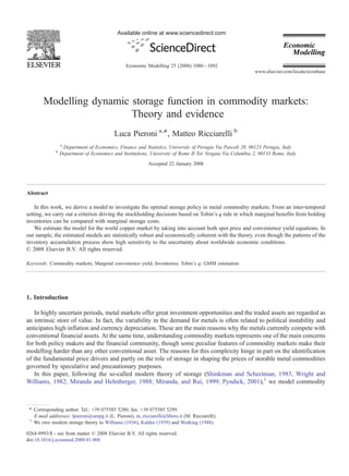
  • 7. 1086 L. Pieroni, M. Ricciarelli / Economic Modelling 25 (2008) 1080–1092 Fig. 1. Spot and futures prices. For the sake of empirical tractability we take into account the discrete time version of equation (Fs) in which the storage level at time t − 1 is used as the initial value, and the optimal rate of inventory accumulation is used to obtain the inventory level at time t. Because the variables involved in q(t) are not determined at time t − 1, we replace the expected value of the endogenous variables P(t) and ϕ(t) according to Eqs. (11) and (13). Thus, we can compute the following recursive algorithm: ̂ Fsðt Þ ¼ Fsðt À 1Þq̂ðt Þ ð19Þ ˆ ˆ where q(t) = q (Fst − 1,Qt − 1)Δt. Focusing on the world copper market, we discuss below our data, the properties of the series and the estimation of the model presented in Section 2. 4. Data and estimation results The model is estimated using monthly data for the world copper market on a time interval ranging from July 1993 to July 2005.7 Hence, changes in the variables of interest will be approximated on a monthly basis.8 In Fig. 1, we present the LME copper spot and futures prices with three-month maturity, respectively. Nominal monthly spot and futures prices, i.e. (P) and (Pf ) are obtained as the averages of the weekly prices recorded in each month and are deflated by means of the US Consumer Price Index (cpi). In order to obtain an estimated series for ϕ, the interest rate (r) herein used is the US three-month Treasury bill rate. Moreover, the dollar index of the real foreign exchange rate (exc) is constructed as a nominal broad dollar index divided by the domestic (US) price level, while prices for Crude Oil are obtained from the London Brent Crude Oil Index (Ctd) and are deflated by the U.S. Producer Price Index ( ppi). 7 The data used in this empirical section are available for replication upon request. 8 This statement is not in contrast with the assumption of a competitive structure of the world copper market. For example, Agostini (2006) shows that, although the US copper industry is highly concentrated and has important sunk costs, the producer prices were close to prices predicted under competitive behaviour.
  • 8. L. Pieroni, M. Ricciarelli / Economic Modelling 25 (2008) 1080–1092 1087 Table 1 Preliminary regressions for convenience yield equations Parameters Estimation of Eq. (13) Generalized estimation of Eq. (13) Baseline model of storage a0 − 38.02 − 2.854 268.48 [0.258] [0.942] [0.000] a1 0.127 0.1197 [0.000] [0.000] a2 − 0.0001 − 0.0002 − 0.0005 [0.000] [0.004] [0.000] a3 − 0.042 − 0.035 [0.716] [0.758] a4 0.11-09 0.25-09 [0.092] [0.001] Notes: the estimated model of column 2 is: ϕ =a0 +a1P(t) +a2Fs(t) +a3σ(t) +e(t). The model shown in column 3 is: ϕ =a0 +a1P(t) +a2Fs(t) +a3σ(t) + a4Fs2(t) +e(t), while the specification in the last column is :ϕ =a0 +a2Fs(t) +a4Fs2(t) +e(t). p-values are reported in brackets. The properties of the time series are investigated by means of the unit root tests. The Dickey and Fuller test corrected by the GLS estimator is employed for the variables of Eqs. (11) and (13) by including the presence/absence of deterministic components. For the sake of robustness, we also carry out the KPSS test in which the null-hypothesis of stationarity is tested against the alternative non-stationarity hypothesis. The results are shown in the data appendix and highlight an overall rejection of the presence of a unit root that justifies the use of the classical methods of estimation for our model.9 By empirically testing the impact of inventories on the copper market, we preliminarily verify the role of storage theory: it suggests that inventories largely affect metal spot prices. Firstly, we estimate the specification of Eq. (13). The results shown in the first column of Table 1 are obtained by the means of the OLS estimator. A significant and linear negative relationship between convenience yield and inventories is documented for agricultural commodities (Brennan, 1958) and for the copper, lumber and heating oil markets (Pindyck, 2004). Secondly, to test for the presence of non-linearities in the relationship, we include a quadratic term in the storage level (2 Fs) in Eq. (13) (Ng and Ruge-Murgia, 1997, p. 12). In this extended specification (see the second column of Table 1), we point out that the quadratic term in the storage does not affect the marginal convenience yield.10 However, this result does not imply a priori the rejection of the storage theory. In fact, a counterfactual test is based on a restricted specification in which marginal convenience yield is regressed on a second order polynomial structure for inventories. While we denote the robustness of the relationship between inventories and marginal convenience yield, the results of the model, shown in column 3, exhibit a positive and significant coefficient for the quadratic term in the inventories (Fs2). From this evidence, we may emphasize that change in copper inventories affects not only the spot price patterns, but also marginal convenience yield in a non-linear manner. Because of the simultaneity between the buy/sell choices in the spot market and the stockholding decisions, the spot price in Eq. (11) generates endogeneity issues and a potential inconsistency of OLS estimators. For this reason, Eqs. (11) and (13) are estimated in a multivariate affine framework, in which we run the instrumental variable estimator via the 3SLS and GMM procedures. In the first column of Table 2, we show the parameters of price and marginal convenience yield equations estimated by 3SLS. The instruments are reported at the bottom of Table 2 and ensure a suitable empirical performance. The estimated parameters are coherent from both an economic and a statistical standpoint. A positive change in stocks reduces the current availability of copper for spot dealings and, hence, has a positive impact on the spot price. Therefore, as pointed out by Chambers and Bailey (1996) and Deaton and Laroque (1992, 1996), storage seems to play a prominent role in affecting the pattern of spot prices in commodity markets. Moreover, a significant and negative coefficient of the exchange rate suggests that those who invest in copper adjust to monetary shocks with significant effects on market transactions (Gilbert, 1989). As expected, the estimated parameter of crude oil has a positive impact on the spot price. The relevance of this input in copper production results into an increase in the marginal cost whose effects are embodied in the spot price. 9 We would like to remark that all time-series variables on the right-hand-side of our equations have shown a stationary process. 10 This coefficient was not significant even when Newey and West standard errors were included in the regression.
  • 9. 1088 L. Pieroni, M. Ricciarelli / Economic Modelling 25 (2008) 1080–1092 Table 2 Estimation results of Eqs. (11) and (13) Parameters 3SLS 3SLS GMM δ0 5436.31 5432.45 5313.62 [21.393] [21.452] [12.106] δ1 0.0021 0.0021 0.0021 [2.608] [2.563] [1.862] δ2 − 42.813 −42.789 − 41.172 [− 16.551] [− 16.61] [−10.87] δ3 8.5274 8.607 7.513 [2.250] [2.282] [1.648] a1 0.075 0.065 0.066 [7.006] [25.32] [12.76] a2 − 0.706-04 −0.657-04 − 0.693-04 [− 7.320] [− 8.219] [−6.626] a3 − 0.2334 [0.909] Price equation R2 = 0.819 R2 = 0.821 R2 = 0.817 Convenience yield equation R2 = 0.772 R2 = 0.788 R2 = 0.787 J-test for over-identifying restrictions 16.7388 [0.160] Notes: t-Student's statistics are reported in parentheses below estimates. The p-value of the J-test is reported in square brackets. Instruments used in estimations are: Constant, Trend, pbrent, pgas, exc, σ (− 1), dFs (− 1), Fs(− 1), P(− 1). The preliminary statistical tests for structural stability of marginal convenience yield Eq. (13) do not show specific shocks, while the estimated coefficients are consistent with the underlying theoretical relationships. Spot prices positively affect marginal convenience yield: as spot prices increase, the convenience of holding a stored unit should increase as well. Stockholdings are negatively related to marginal convenience yield whose value should converge toward zero as the stored amounts tend to infinity. Conversely, the coefficient of spot price volatility is not statistically significant. Thus, a parsimonious specification of the marginal convenience yield equation is carried out by excluding the volatility of copper prices (see column 2 of Table 2). The estimated results confirm the theoretical suggestions and the estimated coefficients are close to those reported in column 1. The outcomes of the diagnostic procedures are consistent with the lack of heteroskedasticity and autocorrelation in both equations. The estimated price equation highlights that the hypothesis of homoskedasticity tested by the LM statistic is rejected for price equation 4.2527 [0.039]. However, as mentioned before, serial correlation problems affect the price pattern. To generalize the serial correlation test, we use a multivariate framework based on Fisher's distribution for finite samples, as derived by Harvey (1990). The empirical value of this testing procedure (F(4,269)) equals 58.96 ( p-value = 0.00) and shows the presence of substantial persistence in the world copper market.11 In order to account for heteroskedasticity and autocorrelation issues, we estimate the copper model by GMM procedure. For the sake of comparability across estimates, the orthogonality conditions are met by holding the set of instruments used in the 3SLS estimations unchanged.12 In the first stage of the GMM estimation, the most significant instruments for the two equations lie on both lagged prices and stocks. Furthermore, the estimates for the spot price equation may be notably improved by using the time trend as an instrument. The fact that the time trend represents a valuable instrument in the spot price equation can be rationalized by the persistence of the copper spot price and has been recently shown by Pieroni and Ricciarelli (2005). In column 3, the results are economically consistent with respect to the previous findings, even if the size of some coefficients can be slightly different. As mentioned above, for each specific combination (Q, Fs), we calculate the optimal storage rate by using the predictions of GMM estimations for spot price and marginal convenience equations. In Fig. 2, we show the optimal storage rate and the aggregate stocks. The values for optimal storage rate (q) are in general less than one with a downward trend to accumulate inventories excluding the months that follow 9/11. In fact, economic agents' behaviour (speculators) readdressed the optimal path of stocks by the positive substitutability effects among assets since the risk 11 In order to strengthen our results, we tested the second order autocorrelation hypothesis. Statistic test F(8,261) is used to compare our empirical results; also in this case, we reject the hypothesis of absence of autocorrelation. 12 To identify the stochastic term, the optimal Andrew's (1991) bandwidth is achieved by five autocorrelation terms.
  • 10. L. Pieroni, M. Ricciarelli / Economic Modelling 25 (2008) 1080–1092 1089 Fig. 2. The estimated stockholding rule and stocks. premium of financial assets led them to be more remunerative than metal markets (Thurman, 1988). As for other commodities, an upward cycle to accumulate inventory from the copper market occurred after the worldwide economic slowdown ignited by 9/11. Price volatility is magnified by the worldwide shock and drives agents to accumulate inventories because of an increasing convenience yield. ˆ Finally, by using the algorithm described in Section 3, the fitted stock values, Fs, are compared with the pattern of Tobin's q. It can be appraised that the computation values of Tobin's q closely track the stockholding behaviour in the world copper market. 5. Concluding remarks In this paper, we derive a model for metal commodity markets from an inter-temporal setting. The optimization problem is herein carried out by the means of the dynamic programming technique in which, for each time period, the market agents can control the levels of production and the amounts of metal commodities to be stored. In comparison with the state of the art, the contribution of this paper is twofold. Firstly, a closed form solution for storage marginal value directly arises from the model and, in turn, by using a measurement equation for marginal convenience yield, we can empirically calculate Tobin's q function. Secondly, from our analytical computations, we can investigate the aggregate behaviour concerning the stockholding strategy of a given commodity. The interpretation of Tobin's q is straightforward and parallels its reading key in the investment theory, namely, to accumulate inventories as marginal benefits from holding inventories exceed marginal storage costs. We use world copper data to test the theoretical model. Estimations of the spot price and marginal convenience yield equations are obtained by 3SLS and GMM procedures. We find that the estimated parameters are statistically robust to different specifications and coherent with theoretical predictions. However, the novelty of the paper lies in showing that optimal continuous time rule for inventory changes is obtained in terms of relative prices, so that an estimated value of Tobin's q of less than one implies a decreasing instantaneous adjustment of inventories. This evidence has been tested
  • 11. 1090 L. Pieroni, M. Ricciarelli / Economic Modelling 25 (2008) 1080–1092 over the period 1993–2005 when demand shocks in the world copper market were intimately related to the business cycle and positive marginal convenience yield reduced stock levels. Only after 9/11, as a result of higher market uncertainty, financial markets recorded a cut in marginal convenience yield, driving economic agents to keep more inventories for precautionary motives. Finally, given the robustness of the results and the good performance of the empirical framework, any extension of our model to different commodity markets and to high frequency data is left for future work. Appendix A. Technical appendix: the derivation of the theoretical model In this technical appendix, we deal with the derivation of the theoretical model introduced in Section 2.2. Let us consider a finite time horizon on [0,T]. We assume that, in each period (t), a representative market agent should maximize an instantaneous profit function by choosing the amount to be produced (Q) and the storage levels (Fs). Thus, by using the lifetime horizon, the objective function of our maximization will be: Z T PðQt ; Fst Þ ¼ e–rðtÞ ½Pðt ÞDðt Þ À TCðt ÞŠdt ðA:1Þ 0 in which P(t) is the spot price, D(t) represents the market demand, which can be also expressed by exploiting the market-clearing condition and, finally, TC(t) stands for the total cost function. Eq. (A.1) parallels the sum of the discounted profits and generalizes such a notion in continuous time. Furthermore, inter-temporal optimization should comply with the stockholding motion law, which can be specified as follows: : Fst ¼ qðFs; Q; t Þdt ðA:2Þ in which ρ(Fs,Q,t) is the key parameter driving changes in inventories over time. In order to solve the optimization program, we should delve into the variables involved in the expression (A.1). In particular, the total cost function needs some clarifications. Following Pindyck (2001), we assume that total cost function results from the sum of the following components: (i) production costs; (ii) marketing costs; and, (iii) stockholding costs. In this setting, we maintain the specifications proposed by Pindyck (2001), namely, the production cost function is specified as quadratic form with respect to the level of production: 1 C ðQðt ÞÞ ¼ ðc0 þ gðt ÞÞQðt Þ þ c1 Qðt Þ2 þc2 Ctdðt ÞQðt Þ ðA:3Þ 2 in which Ctd(t) is the cost for inputs, while η(t) denotes a shock that affects the marginal cost and captures unpredictable changes in the unitary variable cost. Similarly, the marketing cost function can be specified as a quadratic form in the stockholding activities: a2 Uð Pðt Þ; Fsðt Þ; rðt ÞÞ ¼ c0 þ ½Àa0 À a1 Pðt Þ À a3 rðt ÞŠFsðt Þ À Fsðt Þ2 ðA:4Þ 2 in which P(t) and σ(t) stand for spot price and spot price volatility, respectively. Finally, the stockholding cost is assumed to be linear in the stored amounts of inventories: SCðFsðt ÞÞ ¼ kFsðt Þ ðA:5Þ where k denotes the marginal warehousing cost. Once the functional forms for total costs have been specified, we can solve the inter-temporal optimization problem and, hence, we may write the Hamiltonian as: 8 9 ! 1 = Àrðt Þ 2 H ¼e Pðt ÞðQðt Þ þ qð:; t ÞÞ À ðc0 þ gðt ÞÞQðt Þ þ c1 Qðt Þ þc2 Ctdðt ÞQðt Þ þ U½Fsðt Þ; :Š þ kFsðt Þ þ : 2 : ; kðt Þ½qð:; t ÞŠ ðA:6Þ
  • 12. L. Pieroni, M. Ricciarelli / Economic Modelling 25 (2008) 1080–1092 1091 By recalling the definition of marginal convenience yield, i.e. ϕ(t) = −∂Φ(·) / ∂Fs(t), the first order conditions (FOCs) can be carried out as follows: AH ¼ 0 Z Pðt Þ ¼ c0 þ c1 Qðt Þ þ c2 Ctdðt Þ þ gðt Þ ðA:7:aÞ AQðt Þ AH ¼ 0 Z kðt Þ ¼ Pðt Þ À ½/ðt Þ À k Š ðA:7:bÞ AFsðt Þ Price equation (Eq. (A.7.a)) that results from a maximizing behaviour of economic agents can be further mani- pulated by accounting for the demand shifters embedded in the definition for Q (see Eq. (2) in Section 2). From such a manipulation, we may obtain the following equation for the spot price: Pðt Þ ¼ d0 þ d1 dFsðt Þ þ d2 EXCðt Þ þ d3 Ctdðt Þ þ nðt Þ ðA:8Þ in which EXC(t) and Ctd(t) represent two demand shifters, which have received special attention in some previous papers on this topic (Gilbert, 1989), and ξ(t) is an i.i.d. error term. From the second equation (Eq. (A.7.b)), we can obtain a closed form solution for marginal value of a stored amount: it will involve spot price (P(t)), marginal convenience yield (ϕ(t)) and marginal storage cost (k). In order to have some predictive insights on marginal convenience yield, we exploit the specification for marketing costs (Eq. (A.4)) and by using the definition of marginal convenience yield, we obtain: AUðd Þ /ðt Þ ¼ À ¼ a0 þ a1 Pðt Þ þ a2 Fsðt Þ þ a3 rðt Þ þ eðt Þ ðA:9Þ AFsðt Þ in which e(t) stands for an i.i.d. error term, while the other variables have already been mentioned in this appendix. Eqs. (A.7.a) and (A.9) are estimated in the empirical part of this paper and are used to obtain economic agents' predictions on spot price and marginal convenience yield. The predicted values for these variables are plugged into Eq. (A.7.b) to compute the marginal value of storage and, as discussed in the body of this paper, to calculate the value of Tobin's q. Appendix B Data appendix: unit root tests Test Pt ft Fst dFst EXCt Ctdt σt DF(GLS) −1.941⁎⁎ − 1.742⁎ −1.762⁎ − 4.613⁎⁎⁎ − 1.632⁎ − 1.692⁎ − 2.312⁎⁎ KPSS 0.334 0.304 0.218 0.147 0.325 0.342⁎ 0.307 Notes: the critical values of the Dickey–Fuller test (H0 = non-stationarity), corrected by using GLS estimation, are derived by the Elliott– Rothenberg–Stock and tabulated in MacKinnon (1996). Their values are 2.58, 1.94 and 1.61 at the levels of 1%, 5% and 10%, respectively. The asymptotic critical values of Kwiatkowski–Phillips–Schmidt–Shin test (1992) (H0 = stationarity) are 0.79, 0.46 and 0.34 at the levels of 1%, 5% and 10%, respectively. We denote the significance of the test by the number of asterisks: ⁎ (10%), ⁎⁎ (5%) and ⁎⁎⁎ (1%). References Agostini, C., 2006. Estimating market power in the US copper industry. Review of Industrial Organization 28, 17–39. Andrews, D.W.K., 1991. Heteroskedasticity and Autocorrelation Consistent Covariance Matrix Estimation. Econometrica 59, 817–858. Bessembinder, H., Coughenour, J., Seguin, P., Smoller, M., 1995. Mean reversion in equilibrium asset prices: evidence from the futures term structure. Journal of Finance 50, 361–375. Black, F., 1976. The pricing of commodity contracts. Journal of Financial Economics 3, 167–179. Brennan, M.J., 1958. The supply of storage. American Economic Review 48, 50–72. Brennan, M.J., Schwartz, E., 1985. Evaluating natural resource investments. Journal of Business 20, 135–157. Chambers, M.J., Bailey, R.E., 1996. A theory of commodity price fluctuations. Journal of Political Economy 104, 924–957. Casassus, J., Collin-Dufresne, P., 2005. Stochastic convenience yield implied from commodity futures and interest rates. Journal of Finance 60, 2283–2331.
  • 13. 1092 L. Pieroni, M. Ricciarelli / Economic Modelling 25 (2008) 1080–1092 Clewlow, L., Strickland, C., 2000. Energy Derivatives: Pricing and Risk Management. Lacima Publications, London. Deaton, A., Laroque, G., 1992. On the behaviour of commodity prices. Review of Economic Studies 59, 1–23. Deaton, A., Laroque, G., 1996. Competitive storage and commodity price dynamics. Journal of Political Economy 104, 896–923. De Grauwe, P., 1996. International Money: Postwar-Trends and Theories. Oxford University Press, Oxford. Eckstein, Z., Eichenbaum, M.S., 1985. Inventories and Quantity-Constrained Equilibria in Regulated Markets: The US Petroleum Industry, 1947– 1972, in Sargent T, Energy Foresight and Startegy. Resources for the Future, Washington D.C. Fama, E., French, K., 1988. Business cycles and the behaviour of metals prices. Journal of Finance 43, 1075–1093. Gilbert, C.L., 1989. The impact of exchange rates and developing country debt on commodity price. Economic Journal 99, 773–784. Gilbert, C.L., 1995. Modelling market fundamentals: a model of aluminium market. Journal of Applied Econometrics 10, 385–410. Hansen, L., 1982. Large sample properties of generalized method of moments estimators. Econometrica 50, 1029–1054. Hansen, L., Singleton, K.J., 1982. Generalized instrumental variables estimation of nonlinear rational expectations models. Econometrica 50, 1269–1286. Harvey, A., 1990. The Econometric Analysis of Time Series, second ed. MIT Press, Cambridge. Hayashi, F., 1982. Tobin's marginal q and average q: a neoclassical interpretation. Econometrica 50, 213–224. Kaldor, N., 1939. Speculation and economic stability. Review of Economic Studies 7, 1–27. Kwiatkowski, D., Phillips, P.C.B., Schmidt, P., Shin, Y., 1992. Testing the null hypothesis of stationarity against the alternative of a unit root: how sure we are that economic time series have a unit root? Journal of Econometrics 1–3, 159–178. MacKinnon, J.G., 1996. Numerical distribution functions for unit root and cointegration tests. Journal of Applied Econometrics 11 (6), 601–618. Miltersen, K.R., Schwartz, E.S., 1998. Pricing of option on commodity futures with stochastic term structures of convenience yields and interest rates. Journal of Financial and Quantitative Analysis 33, 33–59. Miranda, M.J., Helmberger, P.G., 1988. The effects of price band buffer stocks programs. American Economic Review 78, 46–58. Miranda, M.J., Rui, X., An Empirical Reassessment of the Commodity Storage Model. Working Paper: Ohio State University 1999. Ng, S., Ruge-Murcia, F.J., 1997. Explaining the Persistence of Commodity Price. Department of Economics, Boston College. Nielsen, M.J., Schwartz, E.S., 2004. Theory of storage and the pricing of commodity claims. Review of Derivatives Research 7, 5–24. Pesaran, M.H., 1987. Global and partial non-nested hypotheses and asymptotic local power. Econometric Theory; 12, 69–97. Pesaran, M.H., 1990. An econometric model of exploration and extraction of oil in the UK continental shelf. Economic Journal 100, 367–390. Pieroni, L., Ricciarelli, M., 2005. Testing rational expectations in primary commodity markets. Applied Economics 37, 1705–1718. Pindyck, R.S., 1994. Inventories and short run dynamics of commodity prices. RAND Journal of Economics 25, 141–159. Pindyck, R.S., 2001. The dynamics of commodity spot and futures markets: a primer. The Energy Journal 22, 1–29. Pindyck, R.S., 2004. Volatility and commodity price dynamics. Journal of Futures Market 24, 1029–1047. Pirrong, S.C., Price Dynamics and Derivatives Prices for Continuously produced, storable commodities. Working Paper: University of Washington 1998. Shinkman, J.A., Schectman, J., 1983. A simple competitive model with production and storage. Review of Economic Studies 50, 427–441. Schwartz, E.S., Smith, J.E., 2000. Short-term variation and long-term dynamics in commodity prices. Management Science 46, 893–911. Thurman, W.N., 1988. Speculative carryover: an empirical examination of the U.S. refined copper market. RAND Journal of Economics 19, 420–437. Tobin, J., 1969. A general equilibrium approach to money. Journal of Money, Credit and Banking 1, 15–29. Williams, J.B., 1936. Speculation and the carryover. Quarterly Journal of Economics 50, 436–455. Working, H., 1948. Theory of the inverse carrying charge in futures markets. Journal of Farm Economics 30, 1–28. Wright, B.D., Williams, J.C., 1982. The economic role of commodity storage. Economic Journal 92, 596–614. Wright, B.D., Williams, J.C., 1991. Storage and Commodity Markets. Cambridge University Press, New York.