it has all codes for graphics in R. It starts with basic visualization and then uses ggplot2 package to create colorful graphics

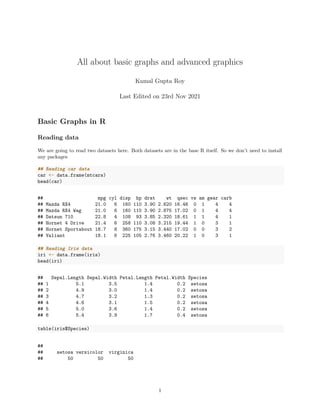
1. All about basic graphs and advanced graphics
Kamal Gupta Roy
Last Edited on 23rd Nov 2021
Basic Graphs in R
Reading data
We are going to read two datasets here. Both datasets are in the base R itself. So we don’t need to install
any packages
## Reading car data
car <- data.frame(mtcars)
head(car)
## mpg cyl disp hp drat wt qsec vs am gear carb
## Mazda RX4 21.0 6 160 110 3.90 2.620 16.46 0 1 4 4
## Mazda RX4 Wag 21.0 6 160 110 3.90 2.875 17.02 0 1 4 4
## Datsun 710 22.8 4 108 93 3.85 2.320 18.61 1 1 4 1
## Hornet 4 Drive 21.4 6 258 110 3.08 3.215 19.44 1 0 3 1
## Hornet Sportabout 18.7 8 360 175 3.15 3.440 17.02 0 0 3 2
## Valiant 18.1 6 225 105 2.76 3.460 20.22 1 0 3 1
## Reading Iris data
iri <- data.frame(iris)
head(iri)
## Sepal.Length Sepal.Width Petal.Length Petal.Width Species
## 1 5.1 3.5 1.4 0.2 setosa
## 2 4.9 3.0 1.4 0.2 setosa
## 3 4.7 3.2 1.3 0.2 setosa
## 4 4.6 3.1 1.5 0.2 setosa
## 5 5.0 3.6 1.4 0.2 setosa
## 6 5.4 3.9 1.7 0.4 setosa
table(iris$Species)
##
## setosa versicolor virginica
## 50 50 50
1

2. Histogram
hist(iris$Sepal.Width)
Histogram of iris$Sepal.Width
iris$Sepal.Width
Frequency
2.0 2.5 3.0 3.5 4.0
0
5
10
15
20
25
30
35
hist(iris$Sepal.Width, col=3) # with colors
2

3. Histogram of iris$Sepal.Width
iris$Sepal.Width
Frequency
2.0 2.5 3.0 3.5 4.0
0
5
10
15
20
25
30
35
hist(iris$Sepal.Width,xlab="xlab",ylab="ylab",main="Main",breaks=10,col="blue") # with labels
3

4. Main
xlab
ylab
2.0 2.5 3.0 3.5 4.0
0
5
10
15
20
25
30
35
Boxplot
boxplot(iris$Sepal.Width) # Simple Box Plot
4

5. 2.0
2.5
3.0
3.5
4.0
boxplot(Sepal.Width ~ Species,iris) # by Species
5

6. setosa versicolor virginica
2.0
2.5
3.0
3.5
4.0
Species
Sepal.Width
boxplot(iris$Sepal.Width ~ iris$Species) # by species but different way of writing
6

7. setosa versicolor virginica
2.0
2.5
3.0
3.5
4.0
iris$Species
iris$Sepal.Width
boxplot(iris$Sepal.Length ~ iris$Species, col=5, varwidth=TRUE) # colors with varied width
7

8. setosa versicolor virginica
4.5
5.5
6.5
7.5
iris$Species
iris$Sepal.Length
boxplot(car$mpg ~ as.character(car$carb),varwidth=TRUE) # colors with varied width
8

9. 1 2 3 4 6 8
10
15
20
25
30
as.character(car$carb)
car$mpg
Scatter Plot
plot(iris$Sepal.Length,iris$Petal.Length) # simple plot
9

10. 4.5 5.0 5.5 6.0 6.5 7.0 7.5 8.0
1
2
3
4
5
6
7
iris$Sepal.Length
iris$Petal.Length
plot(iris$Sepal.Length,iris$Petal.Length,xlab="Sepal Length",ylab="Petal Length", main="Sepal Length Vs
10

11. 4.5 5.0 5.5 6.0 6.5 7.0 7.5 8.0
1
2
3
4
5
6
7
Sepal Length Vs Petal Length
Sepal Length
Petal
Length
plot(iris$Sepal.Length,iris$Petal.Length,xlab="Sepal Length",ylab="Petal Length",main="scatter plot", co
11

12. 4.5 5.0 5.5 6.0 6.5 7.0 7.5 8.0
1
2
3
4
5
6
7
scatter plot
Sepal Length
Petal
Length
pch Values
• pch = 0,square
• pch = 1,circle
• pch = 2,triangle point up
• pch = 3,plus
• pch = 4,cross
• pch = 5,diamond
• pch = 6,triangle point down
• pch = 7,square cross
• pch = 8,star
• pch = 9,diamond plus
• pch = 10,circle plus
• pch = 11,triangles up and down
• pch = 12,square plus
• pch = 13,circle cross
• pch = 14,square and triangle down
• pch = 15, filled square
• pch = 16, filled circle
• pch = 17, filled triangle point-up
• pch = 18, filled diamond
• pch = 19, solid circle
• pch = 20,bullet (smaller circle)
• pch = 21, filled circle blue
• pch = 22, filled square blue
12

13. • pch = 23, filled diamond blue
• pch = 24, filled triangle point-up blue
• pch = 25, filled triangle point down blue
Lines on the scatter Plot
plot(iris$Sepal.Length,iris$Petal.Length,xlab="Sepal Length",ylab="Petal Length",main="scatter plot", co
abline(v=6, col="purple") # verical line
abline(h=6, col="red") # Horizontal line
4.5 5.0 5.5 6.0 6.5 7.0 7.5 8.0
1
2
3
4
5
6
7
scatter plot
Sepal Length
Petal
Length
Mean Lines on Scatter Plot
plot(iris$Sepal.Length,iris$Petal.Length,xlab="Sepal Length",ylab="Petal Length",main="scatter plot", co
abline(v=mean(iris$Sepal.Length),col="blue") # line with mean sepal length
abline(h=mean(iris$Petal.Length),col="pink") # line with mean Petal length
fit <- lm(Petal.Length~Sepal.Length, data=iris) # fitting regression
abline(fit, col="yellow") #linear line
13

14. 4.5 5.0 5.5 6.0 6.5 7.0 7.5 8.0
1
2
3
4
5
6
7
scatter plot
Sepal Length
Petal
Length
R-Square between two variables
summary(lm(Petal.Length~Sepal.Length, data=iris))$r.squared
## [1] 0.7599546
R-square between Petal Length and Sepal Length is 76 %
Cross Tab of all numeric attributes
pairs(iris[,1:4])
14

15. Sepal.Length
2.0
3.0
4.0
4.5 5.5 6.5 7.5
0.5
1.5
2.5 2.0 3.0 4.0
Sepal.Width
Petal.Length
1 2 3 4 5 6 7
0.5 1.5 2.5
4.5
6.0
7.5
1
3
5
7
Petal.Width
Bar Plot
counts <- table(car$carb)
barplot(counts)
15

16. 1 2 3 4 6 8
0
2
4
6
8
10
mm <- tapply(iris$Sepal.Length,iris$Species, mean, na.rm=TRUE)
barplot(mm, horiz=TRUE)
16

17. setosa
versicolor
virginica
0 1 2 3 4 5 6
mm <- tapply(iris$Sepal.Width,iris$Species, median, na.rm=TRUE)
barplot(mm, horiz=FALSE)
17

18. setosa versicolor virginica
0.0
0.5
1.0
1.5
2.0
2.5
3.0
Pie Chart
pie(table(iris$Species))
18

19. setosa
versicolor
virginica
pie(table(car$carb), main="Pie Chart", border="brown")
19

20. 1
2
3
4
6
8
Pie Chart
#pie3D(pie(df$nvar1, labels = df$cvar1,explode=0.1)
#install.packages("plotrix")
library(plotrix)
pie3D(table(car$carb), main="Pie Chart", border="brown", explode=0.2)
20

21. Pie Chart
END of Basic Graphs
21

22. Few Slides on Concept and Background of GGPLOT2 Graphs
22

23. GGPLOT Graphs
Difference between looks of basic and ggplot graphs
library(ggplot2)
# ScatterPlot (Basic vs ggplot2)
23

24. plot(iris$Sepal.Length,iris$Petal.Length) # Plot in Base R
4.5 5.0 5.5 6.0 6.5 7.0 7.5 8.0
1
2
3
4
5
6
7
iris$Sepal.Length
iris$Petal.Length
ggplot(data=iris)
24

25. ggplot(data=iris,aes(y=Sepal.Length, x=Petal.Length))
25

26. 5
6
7
8
2 4 6
Petal.Length
Sepal.Length
ggplot(data=iris,aes(y=Sepal.Length, x=Petal.Length)) + geom_point()
26

27. 5
6
7
8
2 4 6
Petal.Length
Sepal.Length
ggplot(data=iris,aes(y=Sepal.Length, x=Petal.Length, col=Species)) + geom_point()
27

28. 5
6
7
8
2 4 6
Petal.Length
Sepal.Length
Species
setosa
versicolor
virginica
ggplot(data=iris,aes(y=Sepal.Length, x=Petal.Length, shape=Species)) + geom_point()
28

29. 5
6
7
8
2 4 6
Petal.Length
Sepal.Length
Species
setosa
versicolor
virginica
ggplot(data=iris,aes(y=Sepal.Length, x=Petal.Length, shape=Species, col=Species)) + geom_point()
29

30. 5
6
7
8
2 4 6
Petal.Length
Sepal.Length
Species
setosa
versicolor
virginica
mtcars ggplot histogram
hist(mtcars$mpg)
30

31. Histogram of mtcars$mpg
mtcars$mpg
Frequency
10 15 20 25 30 35
0
2
4
6
8
10
12
ggplot(mtcars, aes(x = mpg)) + geom_histogram(binwidth = 5)
31

32. 0
3
6
9
10 20 30
mpg
count
All about ggplot2
Libraries for ggplot2 and Manipulation
library(dplyr)
##
## Attaching package: ’dplyr’
## The following objects are masked from ’package:stats’:
##
## filter, lag
## The following objects are masked from ’package:base’:
##
## intersect, setdiff, setequal, union
library(ggplot2)
house <- read.csv("C:UserskamalDropbox (Erasmus Universiteit Rotterdam)Kamal GuptaAMSOM-Teachi
32

33. head(house)
## X price lot_size waterfront age land_value construction air_cond fuel
## 1 1 132500 0.09 No 42 50000 No No Electric
## 2 2 181115 0.92 No 0 22300 No No Gas
## 3 3 109000 0.19 No 133 7300 No No Gas
## 4 4 155000 0.41 No 13 18700 No No Gas
## 5 5 86060 0.11 No 0 15000 Yes Yes Gas
## 6 6 120000 0.68 No 31 14000 No No Gas
## heat sewer living_area fireplaces bathrooms rooms
## 1 Electric Private 906 1 1.0 5
## 2 Hot Water Private 1953 0 2.5 6
## 3 Hot Water Public 1944 1 1.0 8
## 4 Hot Air Private 1944 1 1.5 5
## 5 Hot Air Public 840 0 1.0 3
## 6 Hot Air Private 1152 1 1.0 8
str(house)
## ’data.frame’: 1728 obs. of 15 variables:
## $ X : int 1 2 3 4 5 6 7 8 9 10 ...
## $ price : int 132500 181115 109000 155000 86060 120000 153000 170000 90000 122900 ...
## $ lot_size : num 0.09 0.92 0.19 0.41 0.11 0.68 0.4 1.21 0.83 1.94 ...
## $ waterfront : chr "No" "No" "No" "No" ...
## $ age : int 42 0 133 13 0 31 33 23 36 4 ...
## $ land_value : int 50000 22300 7300 18700 15000 14000 23300 14600 22200 21200 ...
## $ construction: chr "No" "No" "No" "No" ...
## $ air_cond : chr "No" "No" "No" "No" ...
## $ fuel : chr "Electric" "Gas" "Gas" "Gas" ...
## $ heat : chr "Electric" "Hot Water" "Hot Water" "Hot Air" ...
## $ sewer : chr "Private" "Private" "Public" "Private" ...
## $ living_area : int 906 1953 1944 1944 840 1152 2752 1662 1632 1416 ...
## $ fireplaces : int 1 0 1 1 0 1 1 1 0 0 ...
## $ bathrooms : num 1 2.5 1 1.5 1 1 1.5 1.5 1.5 1.5 ...
## $ rooms : int 5 6 8 5 3 8 8 9 8 6 ...
summary(house)
## X price lot_size waterfront
## Min. : 1.0 Min. : 5000 Min. : 0.0000 Length:1728
## 1st Qu.: 432.8 1st Qu.:145000 1st Qu.: 0.1700 Class :character
## Median : 864.5 Median :189900 Median : 0.3700 Mode :character
## Mean : 864.5 Mean :211967 Mean : 0.5002
## 3rd Qu.:1296.2 3rd Qu.:259000 3rd Qu.: 0.5400
## Max. :1728.0 Max. :775000 Max. :12.2000
## age land_value construction air_cond
## Min. : 0.00 Min. : 200 Length:1728 Length:1728
## 1st Qu.: 13.00 1st Qu.: 15100 Class :character Class :character
## Median : 19.00 Median : 25000 Mode :character Mode :character
## Mean : 27.92 Mean : 34557
## 3rd Qu.: 34.00 3rd Qu.: 40200
## Max. :225.00 Max. :412600
33

34. ## fuel heat sewer living_area
## Length:1728 Length:1728 Length:1728 Min. : 616
## Class :character Class :character Class :character 1st Qu.:1300
## Mode :character Mode :character Mode :character Median :1634
## Mean :1755
## 3rd Qu.:2138
## Max. :5228
## fireplaces bathrooms rooms
## Min. :0.0000 Min. :0.0 Min. : 2.000
## 1st Qu.:0.0000 1st Qu.:1.5 1st Qu.: 5.000
## Median :1.0000 Median :2.0 Median : 7.000
## Mean :0.6019 Mean :1.9 Mean : 7.042
## 3rd Qu.:1.0000 3rd Qu.:2.5 3rd Qu.: 8.250
## Max. :4.0000 Max. :4.5 Max. :12.000
Histogram
ggplot(data=house, aes(x=price/100000)) + geom_histogram()
## ‘stat_bin()‘ using ‘bins = 30‘. Pick better value with ‘binwidth‘.
0
100
200
0 2 4 6 8
price/1e+05
count
34

35. ggplot(data=house, aes(x=price/100000)) + geom_histogram(bins=50)
0
50
100
150
0 2 4 6 8
price/1e+05
count
ggplot(data=house, aes(x=price/100000)) + geom_histogram(bins=50,fill="palegreen4")
35

36. 0
50
100
150
0 2 4 6 8
price/1e+05
count
ggplot(data=house, aes(x=price/100000)) + geom_histogram(bins=50,fill="palegreen4", col="green")
36

37. 0
50
100
150
0 2 4 6 8
price/1e+05
count
##############################
ggplot(data=house, aes(x=price/100000)) + geom_histogram()
## ‘stat_bin()‘ using ‘bins = 30‘. Pick better value with ‘binwidth‘.
37

38. 0
100
200
0 2 4 6 8
price/1e+05
count
ggplot(data=house, aes(x=price/100000)) + geom_histogram(bins=50)
38

39. 0
50
100
150
0 2 4 6 8
price/1e+05
count
ggplot(data=house, aes(x=price/100000,fill=air_cond)) + geom_histogram(bins=50)
39

40. 0
50
100
150
0 2 4 6 8
price/1e+05
count
air_cond
No
Yes
ggplot(data=house, aes(x=price/100000,fill=air_cond)) + geom_histogram(bins=50,position="fill")
## Warning: Removed 8 rows containing missing values (geom_bar).
40

41. 0.00
0.25
0.50
0.75
1.00
0 2 4 6 8
price/1e+05
count
air_cond
No
Yes
ggplot(data=house, aes(x=price/100000,fill=air_cond)) + geom_histogram(bins=50,position="identity")
41

42. 0
25
50
75
100
125
0 2 4 6 8
price/1e+05
count
air_cond
No
Yes
Bar Plot
ggplot(data=house, aes(x=waterfront)) + geom_bar()
42

43. 0
500
1000
1500
No Yes
waterfront
count
ggplot(data=house, aes(x=waterfront,fill=air_cond)) + geom_bar()
43

44. 0
500
1000
1500
No Yes
waterfront
count
air_cond
No
Yes
ggplot(data=house, aes(x=waterfront,fill=air_cond)) + geom_bar(position="fill")
44

45. 0.00
0.25
0.50
0.75
1.00
No Yes
waterfront
count
air_cond
No
Yes
ggplot(data=house, aes(x=waterfront,fill=sewer)) + geom_bar()
45

46. 0
500
1000
1500
No Yes
waterfront
count
sewer
None
Private
Public
ggplot(data=house, aes(x=waterfront,fill=sewer)) + geom_bar(position="fill")
46

47. 0.00
0.25
0.50
0.75
1.00
No Yes
waterfront
count
sewer
None
Private
Public
Frequency Polygon
ggplot(data=house, aes(x=price/100000)) + geom_freqpoly()
## ‘stat_bin()‘ using ‘bins = 30‘. Pick better value with ‘binwidth‘.
47

48. 0
100
200
0 2 4 6 8
price/1e+05
count
ggplot(data=house, aes(x=price/100000)) + geom_freqpoly(bins=60)
48

49. 0
50
100
0 2 4 6 8
price/1e+05
count
ggplot(data=house, aes(x=price/100000, col=air_cond)) + geom_freqpoly(bins=60)
49

50. 0
25
50
75
100
0 2 4 6 8
price/1e+05
count
air_cond
No
Yes
ggplot(data=house, aes(x=price/100000)) + geom_freqpoly(size=2, bins=50,col="blue")
50

51. 0
50
100
150
0 2 4 6 8
price/1e+05
count
Box Plot
ggplot(data=house, aes(x=factor(rooms),y=price)) + geom_boxplot()
51

52. 0e+00
2e+05
4e+05
6e+05
8e+05
2 3 4 5 6 7 8 9 10 11 12
factor(rooms)
price
ggplot(data=house, aes(x=factor(rooms),y=price, fill=factor(rooms))) + geom_boxplot()
52

53. 0e+00
2e+05
4e+05
6e+05
8e+05
2 3 4 5 6 7 8 9 10 11 12
factor(rooms)
price
factor(rooms)
2
3
4
5
6
7
8
9
10
11
12
ggplot(data=house, aes(x=factor(rooms),y=price, fill=air_cond)) + geom_boxplot()
53

54. 0e+00
2e+05
4e+05
6e+05
8e+05
2 3 4 5 6 7 8 9 10 11 12
factor(rooms)
price
air_cond
No
Yes
ggplot(data=house, aes(x=factor(rooms),y=price, fill=sewer)) + geom_boxplot()
54

55. 0e+00
2e+05
4e+05
6e+05
8e+05
2 3 4 5 6 7 8 9 10 11 12
factor(rooms)
price
sewer
None
Private
Public
Smooth Lines
ggplot(data=house, aes(y=price, x=living_area)) + geom_smooth()
## ‘geom_smooth()‘ using method = ’gam’ and formula ’y ~ s(x, bs = "cs")’
55

56. 2e+05
4e+05
6e+05
1000 2000 3000 4000 5000
living_area
price
ggplot(data=house, aes(y=price, x=living_area)) + geom_smooth(se=F)
## ‘geom_smooth()‘ using method = ’gam’ and formula ’y ~ s(x, bs = "cs")’
56

57. 1e+05
2e+05
3e+05
4e+05
5e+05
6e+05
1000 2000 3000 4000 5000
living_area
price
ggplot(data=house, aes(y=price, x=living_area, col=air_cond)) + geom_smooth(se=F)
## ‘geom_smooth()‘ using method = ’gam’ and formula ’y ~ s(x, bs = "cs")’
57

58. 1e+05
2e+05
3e+05
4e+05
5e+05
6e+05
1000 2000 3000 4000 5000
living_area
price
air_cond
No
Yes
ggplot(data=house, aes(y=price, x=living_area, col=heat)) + geom_smooth(se=F)
## ‘geom_smooth()‘ using method = ’gam’ and formula ’y ~ s(x, bs = "cs")’
58

59. 1e+05
2e+05
3e+05
4e+05
5e+05
6e+05
1000 2000 3000 4000 5000
living_area
price
heat
Electric
Hot Air
Hot Water
Scatter Plot with smooth Lines
ggplot(data=house, aes(y=price, x=living_area)) + geom_point() + geom_smooth(method=lm)
## ‘geom_smooth()‘ using formula ’y ~ x’
59

60. 0e+00
2e+05
4e+05
6e+05
8e+05
1000 2000 3000 4000 5000
living_area
price
ggplot(data=house, aes(y=price, x=living_area)) + geom_point() + geom_smooth(method=lm, se=F)
## ‘geom_smooth()‘ using formula ’y ~ x’
60

61. 0e+00
2e+05
4e+05
6e+05
8e+05
1000 2000 3000 4000 5000
living_area
price
ggplot(data=house, aes(y=price, x=living_area, col=air_cond)) + geom_point() + geom_smooth(method=lm, se
## ‘geom_smooth()‘ using formula ’y ~ x’
61

62. 0e+00
2e+05
4e+05
6e+05
8e+05
1000 2000 3000 4000 5000
living_area
price
air_cond
No
Yes
Scatter Plot with smooth Lines with facets
ggplot(data=house, aes(y=price, x=living_area, col=air_cond)) + geom_point() +
geom_smooth(method=lm, se=F) + facet_grid(~air_cond)
## ‘geom_smooth()‘ using formula ’y ~ x’
62

63. No Yes
1000 2000 3000 4000 5000 1000 2000 3000 4000 5000
0e+00
2e+05
4e+05
6e+05
8e+05
living_area
price
air_cond
No
Yes
ggplot(data=house, aes(y=price, x=living_area, col=factor(fireplaces))) + geom_point() +
geom_smooth(method=lm, se=F) + facet_grid(~fireplaces)
## ‘geom_smooth()‘ using formula ’y ~ x’
63

64. 0 1 2 3 4
1000
2000
3000
4000
5000
1000
2000
3000
4000
5000
1000
2000
3000
4000
5000
1000
2000
3000
4000
5000
1000
2000
3000
4000
5000
0e+00
2e+05
4e+05
6e+05
8e+05
living_area
price
factor(fireplaces)
0
1
2
3
4
ggplot(data=house, aes(y=price, x=age, col=factor(fireplaces))) + geom_point() + geom_smooth(method=lm,
## ‘geom_smooth()‘ using formula ’y ~ x’
64

65. 0 1 2 3 4
0 50100
150
200 0 50100
150
200 0 50100
150
200 0 50100
150
200 0 50100
150
200
0e+00
2e+05
4e+05
6e+05
8e+05
age
price
factor(fireplaces)
0
1
2
3
4
Themes
#install.packages("scales")
library(scales)
##
## Attaching package: ’scales’
## The following object is masked from ’package:plotrix’:
##
## rescale
ob1 <- ggplot(data=house, aes(x=factor(rooms),y=price, fill=factor(rooms))) + geom_boxplot()
ob2 <- ob1 + labs(title="Price w.r.t number of rooms", subtitle = "Boxplot", x="Number of Rooms", y="Pri
ob3 <- ob2 + theme(panel.background = element_rect("palegreen1"))
ob4 <- ob3 + theme(plot.title = element_text(hjust=0.5,face="bold",colour = "cadetblue"))
ob4 + scale_y_continuous(labels = dollar)
65

66. $0
$200,000
$400,000
$600,000
$800,000
2 3 4 5 6 7 8 9 10 11 12
Number of Rooms
Price
of
a
House
factor(rooms)
2
3
4
5
6
7
8
9
10
11
12
Boxplot
Price w.r.t number of rooms
Corelogram
#install.packages("corrplot")
library(corrplot)
## corrplot 0.92 loaded
correlations <- cor(house[,c("price","lot_size","age","land_value","living_area", "fireplaces","bathroom
corrplot(correlations, method="circle")
66

67. −1
−0.8
−0.6
−0.4
−0.2
0
0.2
0.4
0.6
0.8
1
price
lot_size
age
land_value
living_area
fireplaces
bathrooms
rooms
price
lot_size
age
land_value
living_area
fireplaces
bathrooms
rooms
corrplot(correlations, type = "upper", order = "hclust", tl.col = "black", tl.srt = 45)
67

68. −1
−0.8
−0.6
−0.4
−0.2
0
0.2
0.4
0.6
0.8
1
a
g
e
l
o
t
_
s
i
z
e
l
a
n
d
_
v
a
l
u
e
f
i
r
e
p
l
a
c
e
s
l
i
v
i
n
g
_
a
r
e
a
r
o
o
m
s
p
r
i
c
e
b
a
t
h
r
o
o
m
s
age
lot_size
land_value
fireplaces
living_area
rooms
price
bathrooms
round(correlations,2)
## price lot_size age land_value living_area fireplaces bathrooms
## price 1.00 0.16 -0.19 0.58 0.71 0.38 0.60
## lot_size 0.16 1.00 -0.02 0.06 0.16 0.09 0.08
## age -0.19 -0.02 1.00 -0.02 -0.17 -0.17 -0.36
## land_value 0.58 0.06 -0.02 1.00 0.42 0.21 0.30
## living_area 0.71 0.16 -0.17 0.42 1.00 0.47 0.72
## fireplaces 0.38 0.09 -0.17 0.21 0.47 1.00 0.44
## bathrooms 0.60 0.08 -0.36 0.30 0.72 0.44 1.00
## rooms 0.53 0.14 -0.08 0.30 0.73 0.32 0.52
## rooms
## price 0.53
## lot_size 0.14
## age -0.08
## land_value 0.30
## living_area 0.73
## fireplaces 0.32
## bathrooms 0.52
## rooms 1.00
68