Book Typesetting

1. ch-13 NKR/LaTeX Sample (Typeset by TYINDEX, Delhi) 1 of 17 May 31, 2009 17:29
13
SIGNIFICANT TESTS
A fter any experiment we get some results, but we are not sure
about this result whether the result occurred by chance or a real
difference. That time to find truth we will use some statistical tests,
these tests are termed as, ‘Tests of Significance’.
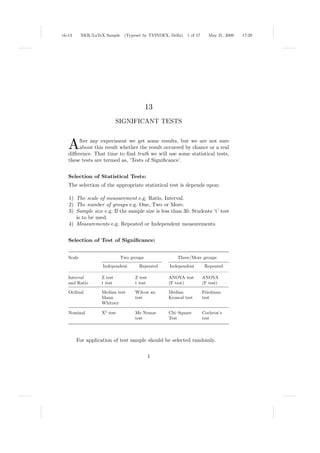
Selection of Statistical Tests:
The selection of the appropriate statistical test is depends upon:
1) The scale of measurement e.g. Ratio, Interval.
2) The number of groups e.g. One, Two or More.
3) Sample size e.g. If the sample size is less than 30. Students ‘t’ test
is to be used.
4) Measurements e.g. Repeated or Independent measurements.
Selection of Test of Significance:
Scale Two groups Three/More groups
Independent Repeated Independent Repeated
Interval Z test Z test ANOVA test ANOVA
and Ratio t test t test (F test) (F test)
Ordinal Median test Wilcox an Median Friedman
Mann test Kruscal test test
Whitney
Nominal X2 test Me Nemar Chi–Square Cochron’s
test Test test
For application of test sample should be selected randomly.
1

2. ch-13 NKR/LaTeX Sample (Typeset by TYINDEX, Delhi) 2 of 17 May 31, 2009 17:29
2 SIGNIFICANT TESTS
There are two types of tests:
1) Parametric Tests
2) Non – Parametric Tests
1. Parametric Test:
When quantitative data like Weight, Length, Height, and Percentage
is given it is used. These tests were based on the assumption that
samples were drawn from the normally distributed populations.
E.g. Students t test, Z test etc.
2. Non – Parametric Test:
When qualitative data like Health, Cure rate, Intelligence, Color is
given it is used. Here observations are classified into a particular
category or groups.
E.g. Chi square (x2 ) test, Median tests etc.
I) T – Test:
W.S. Gosset investigated this test in 1908. It is called Student t –
Test because the pen name of Dr. Gosset was student, hence this test
is known as student’s t – test. It is also called as ‘t- ratio’ because it
is a ratio of difference between two means.
Aylmer Fisher (1890–1962) developed students ‘t’ test where sam-
ples are drawn from normal population and are randomly selected.
After comparing the calculated value of ‘t’ with the value given
in the ‘t’ table considering degree of freedom we can ascertain its
significance.
Patients Before After
treatment (B) treatment (A)
1 2.4 2.2
2 2.8 2.6
3 3.2 3.0
4 6.4 4.2
5 4.3 2.2
6 2.2 2.0
7 6.2 4.8
8 4.2 2.4
Is the testing reliable?

3. ch-13 NKR/LaTeX Sample (Typeset by TYINDEX, Delhi) 3 of 17 May 31, 2009 17:29
SIGNIFICANT TESTS 3
Solution:
Patients Before After Difference D2
treatment (B) treatment (A) B−A=D
1 2.4 2.2 0.2 0.04
2 2.8 2.6 0.2 0.04
3 3.2 3.0 0.2 0.04
4 6.4 4.2 2.2 4.84
5 4.3 2.2 2.1 4.41
6 2.2 2.0 0.2 0.04
7 6.2 4.8 1.4 1.96
8 4.2 2.4 1.8 3.24
D = 8.3 D2 = 14.61
Here,
D = 8.3
N=8
D2 = 14.61
8.3
D= = 1.0375
8
∴ Standard deviation of the different between means.
( D)2
D2 − n
=
N−1
(8.3)2
14.61 − 8
=
7
14.61 − 68.89
8
=
7
14.61 − 8.6112
∴ S.D. =
7
√
= 0.8569
∴ S.D. = 0.9257

4. ch-13 NKR/LaTeX Sample (Typeset by TYINDEX, Delhi) 4 of 17 May 31, 2009 17:29
4 SIGNIFICANT TESTS
Now, standard error of the difference (SED )
SD 0.9257 0.9257
.= √ = √ =
N 8 2.8284
∴ S.E. = 0.3272
D 1.0375
∴t= = = 3.1708
SED 0.3272
Here, the calculated value for ‘t’ exceeds the tabulated ‘t’ value
at p = 0.05 level with 7df. Therefore the glucose concentration by the
patients after treatment is not significant.
Utility:
It is widely used in the field of Medical science, Agriculture and
Veterinary as follows:
r To compare the results of two drugs which is given to same
individuals in the sample at two different situations? E.g. Effect
of Bryonia and Lycopodium on general symptoms like sleep,
appetite etc.
r It is used to study of drug specificity on a particular organ /
tissue / cell level. E.g. Effect of Belberis Vulg. on renal system.
r It is used to compare results of two different methods. E.g.
Estimation of Hb% by Sahlis method and Tallquist method.
r To compare observations made at two different sites of the same
body. E.g. compare blood pressure of arm and thigh.
r To study the accuracy of two different instruments like Ther-
mometer, B.P apparatus etc.
r To accept the Null Hypothesis that is no difference between the
two means.
r To reject the hypothesis that is the difference between the means
of the two samples is statistically significant.
F – Test:
A statistician R.A. Fisher introduces it. That is why it is also called
as Fisher’s test (F – test) test.

5. ch-13 NKR/LaTeX Sample (Typeset by TYINDEX, Delhi) 5 of 17 May 31, 2009 17:29
SIGNIFICANT TESTS 5
Definition: It is the ratio of two independent chi-square variables
which is derived by dividing each by its corresponding degree of
freedom.
Ψ1 2
V1
∴F=
Ψ2 2
V2
Here, two variances are derived from two samples. The values in
each group are to be normally distributed. Therefore the variation of
each value around its group mean that is error is remain independent
of each value provided the variances within each group should be
equal for all groups.
Calculation for F Test:
Tests of hypothesis about the variance of two populations:-
Steps:-
1) Null hypothesis should be H0 = 61 2 = 62 2 and Alternative hypo-
thesis H0 = 61 2 = 62 2 (two tailed test)
2) Calculation of F test statistic:-
61 2
F= if, 61 2 ≥ 62 2
62 2
OR
62 2
F= if, 62 2 ≥ 61 2
61 2
3) Take the level of significance α = 0.05
If α is not known.
Rules for Significance:
1) If calculated F < tabled Fα2 then accept H0 .
2) If, calculated F > tabled Fα2 then reject H0 .

6. ch-13 NKR/LaTeX Sample (Typeset by TYINDEX, Delhi) 6 of 17 May 31, 2009 17:29
6 SIGNIFICANT TESTS
Steps for One Tailed Test:
1. Set the Null Hypothesis (H0 ): 61 2 > 62 2 in such a way that
the rejection appeases in the upper tail by numbering the population
variance.
Format: H0 : 62 2 < 61 2
If, H0 is of the form 61 2 < 62 2 then we calculate F = 61 2 /62 2 which
has F – distribution but with n2 − 1 d.f. in the numerator and n − 1
d.f. in the denominator.
2. Calculation of test statistics:
61 2
∴ F statistics =
62 2
3. Set the level of significance α= 0.05 if value of α is not
known to us.
4. Rules for Significance:
If calculated F α table F2 α then accept the null hypothesis H0 and
reject H0 if calculated F > table Fα.
Example:
1) Random samples are drawn from the two sets of students and the
following results were obtained.
Sample A: 10, 12, 18, 14, 16, 20.
Sample B: 14, 16, 20, 18, 21, 22.
Find the variance of two populations and test whether the two
samples have same variance.
Solution: Null hypothesis H0 = 6A 2 = 6B 2 that is the two samples
have the same variance.
Alternative hypothesis H0: 6A 2 = 6B 2 (Two tailed test)

7. ch-13 NKR/LaTeX Sample (Typeset by TYINDEX, Delhi) 7 of 17 May 31, 2009 17:29
SIGNIFICANT TESTS 7
Calculation of test statistic:
We have the following table to evaluation 6A 2 and 6B 2
A A – A (A – A)2 B – B (B – B)2
(A – 15) (A – 15)2 B (B – 18.5) (B – 18.5)2
10 −5 25 14 −4.5 20.25
12 −3 9 16 −2.5 6.25
18 3 9 20 1.5 2.25
14 −1 1 18 −0.5 0.25
16 1 1 21 2.5 6.25
20 5 25 22 3.5 12.25
A = 90 (A − A)2 B = 111 (B − B)2
= 70 = 47.5
90
We know, A= = 15.
6
Rule of Significance:
1) If, the calculated value of ‘t’ is higher than the value given at
P = 0.05 (5% level) in the table it is significant.
2) If the calculated value of ‘t’ is less than the value given in ‘t’ table
it is not significant.
Degree of Freedom:
It is the quantity in a series which is one less than the independent
number of observations in a sample is called – Degree of freedom.
E.g. In unpaired t test df = N − 1 and in paired t test df =
N1 + N2 − 2 (Where, N1 and N2 are the number of observations.)
There are two types of t – test:
a) Unpaired t – Test.
b) Paired t – Test.
A] Unpaired t – Test:
Indications for Unpaired t – Test:
i) When, samples drawn from two population
OR

8. ch-13 NKR/LaTeX Sample (Typeset by TYINDEX, Delhi) 8 of 17 May 31, 2009 17:29
8 SIGNIFICANT TESTS
When, unpaired data of independent observations of two different
groups are given.
Calculation for Significance Tests:
Following steps are taken to test the significance of difference.
Steps:
1) Find the observed difference between means of two samples.
(X1 − X2 )
2) Calculate the SE of difference between means or SEn .
61 2 62 2
That is S (X1 − X2 ) = +
N1 N2
3) Apply formula for t
(X1 − X2 )
That is t =
61 2 62 2
+
N1 N2
4) Find the degree of freedom.
Example: 1) Raulfia Ø is given to each of the 8 patients resulted in
the following changes in the Blood pressure from normal.
−5, 3, 4, −2, 7, 3, 0, 2
Calculate by students ‘t’ – test whether changes is significant or not.
Solution:
Calculation of mean:
X
∴X=
N
12
=
8
= 1.5

9. ch-13 NKR/LaTeX Sample (Typeset by TYINDEX, Delhi) 9 of 17 May 31, 2009 17:29
SIGNIFICANT TESTS 9
Calculation of S.D:
X X–X=x x2
−5 −5 − 1.5 = −6.5 42.25
3 3 − 1.5 = 1.5 2.25
4 4 − 1.5 = 2.5 6.25
−2 −2 − 1.5 = −3.5 12.25
7 7 − 1.5 = 5.5 30.25
3 3 − 1.5 = 1.5 2.25
0 0 − 1.5 = −1.5 2.25
2 2 − 1.5 = 0.5 0.25
N=8 x2 = 98
x2
∴ = S.D. =
N−1
98 √
= = 14 = 3.74
7
√
X× N
Now, t =
S.D.
1.5 × 2.82
=
3.74
= 1.13
Degree of freedom = N − 1
= 8−1
=7
Here, calculated value of ‘t’ is less than the given value in t table
hence the difference between the two means is significant.
E.g. 2) The weight of an untreated group of six persons are 60kg,
40kg, 45kg, 50kg, 65kg, 70kg. The weight of another group persons
from the same population other treatment with Phytolacca drug was
obtained as, 45kg, 35kg, 40kg, 45kg, 60kg, 65kg and 45 kg. Apply t
test to find out significance of difference between means of two groups.

10. ch-13 NKR/LaTeX Sample (Typeset by TYINDEX, Delhi) 10 of 17 May 31, 2009 17:29
10 SIGNIFICANT TESTS
Solution:
Calculation of Mean:
Untreated Persons Weight X1 X1 − X1 = x x1 2
1 60 60 − 55 = 5 25
2 40 40 − 55 = −15 225
3 45 45 − 55 = −10 100
4 50 50 − 55 = −5 25
5 65 65 − 55 = 10 100
6 70 70 − 55 = 15 225
X1 = 330 x1 2 = 700
X1
∴ Mean of first group = X1 =
N1
330
=
6
= 55
Treated persons Weight X2 X2 − X2 = x2 x2 2
1 45 45 − 47.85 = −2.85 8.12
2 35 35 − 47.85 = −12.85 165.12
3 40 40 − 47.85 = −7.85 61.62
4 45 45 − 47.85 = −2.85 8.12
5 60 60 − 47.85 = 12.15 147.62
6 65 65 − 47.85 = 17.15 294.12
7 45 45 − 47.85 = −2.85 8.12
N2 = 7 X2 = 335 x2 2 = 692.84
X2
And Mean of 2nd group = X2 =
N1
335
=
7
= 47.85

11. ch-13 NKR/LaTeX Sample (Typeset by TYINDEX, Delhi) 11 of 17 May 31, 2009 17:29
SIGNIFICANT TESTS 11
Now, calculate combined S.D. by applying formula:
(x1− X1 )2 + (x2 − X2 )2
∴ Combined S.D. =
N1 + N2 − 2
√
700 + 692.84
=
6+7−2
1392.87
=
11
∴ S.D. = 11.25
Calculation of ‘t’ by applying following formula:
X1 − X2
∴t=
N1 + N2
6
N1 + N2
55 − 47.85
=
6+7
11.25
6+7
7.15
=
13
11.25 ×
13
7.15
∴t= √
11.25 × 1
7.15
=
11.25 × 1
∴ t = 0.635
Here, the calculated value for t. (0.635) is more than that given in
the ‘t’ table for degree of freedom N = (N1 + N2 − 2 = 6 + 7 − 2 =
11). Hence, the difference between two means is not significant.

12. ch-13 NKR/LaTeX Sample (Typeset by TYINDEX, Delhi) 12 of 17 May 31, 2009 17:29
12 SIGNIFICANT TESTS
b] Paired ‘t’– Test:
Indications for Paired t – Test:
i) When paired data of independent observation from one sample
only given.
Calculation for Significance Test:
Following steps are to be taken to test the significance of difference.
Steps:
1) Find the difference in each set of paired observations before and
after treatment (X1 − X2 ) = x.
2) Calculation of Mean of Difference that is x.
S.D.
3) Calculate S.D. of difference and S.E. of Mean from the same √
N
X−0 X
4) Apply formula for ‘t’ that is t = =
5 SEd
√
N
5) Find the degree of freedom.
Example: 1. Two research centers carry out independent estimates
of calcium carbonate content for water made by a certain firm. A
sample is taken from each place and sent to the two centers separately.
They obtain the following results.
Percentage of Calc. Carbonate content in water.
Place No. 1 2 3 4
Center A 8 5 6 3
Center B 6 6 5 4
Is the testing reliable?
Solution:
Ho; µD = 0
Here, the testing will be reliable if the mean difference between
the results from the two-research centers does not differ significantly
form zero. So we assume the hypothesis that the observed differences
are the random observations from a population with mean zero.

13. ch-13 NKR/LaTeX Sample (Typeset by TYINDEX, Delhi) 13 of 17 May 31, 2009 17:29
SIGNIFICANT TESTS 13
Calculation of mean difference and standard error:
Place No. Center Diff. of results
Center A Center B D=B−A D2
1 8 6 −2 4
2 5 6 1 1
3 6 5 −1 1
4 3 4 1 1
Total 22 21 −1 7
−1
Here, D = 4 = −0.25 and µ = 0
( D)2
(D − D)2 = D2 −
N
(−1)2
= 7−
4
(−2)
= 7−
4
= 7 − (−0.5)
= 6, 5
(D − D)
∴ S.E of D =
N(N − 1)
6.5
=
4(4 − 1)
6.5
=
12
= 0.735
D−µ −0.25 − 0
∴t= = = −0.340
S.E. of D 0.735
D.f. = 4 − 1 − 3.

14. ch-13 NKR/LaTeX Sample (Typeset by TYINDEX, Delhi) 14 of 17 May 31, 2009 17:29
14 SIGNIFICANT TESTS
Since the observed value of the t = (− 0.340) is less then the value
of t at 5% level of significance for 3 df. So it is non significant. Hence
the hypothesis will be accepted that is the testing is reliable.
Example 2. The effect of Synz. Jamb. drug on 8 patients showed
concentration of glucose (mg/hr) after 24 hrs as follows:
111 x
B= = 18.5 we know x = n
6
(A − A)2 70
∴ 61 2 = = = 14
n1 − 1 5
(B − B)2 47.5
∴ 62 2 = = = 9.5
n2 − 1 5
62 2 9.5
∴ Test statistics: F = = = 0.6785
61 2 14
Conclusion:
The calculation value of F = 0.6785,
< Table value F 0.05 the null hypothesis H0 is accepted.
∴ The two samples have the same variance.
Testing the Homogeneity of Variance between Groups:
We have following formula,
Largest Variance
∴F=
Smallest Variance
Where the ratio is directly proportional to its significance. E.g.
Standard Deviation was in three groups of students for their marks in
statistics conclude the variance between groups significantly differing
from each other.
Sr. No. Group (1) Group (2) Group (3)
1 Sample size N=10 N= 13 N = 15
2 Standard deviation 0.2757 1.213 0.5512
3 Variance (SD)2 0.076 1.47 0.303

15. ch-13 NKR/LaTeX Sample (Typeset by TYINDEX, Delhi) 15 of 17 May 31, 2009 17:29
SIGNIFICANT TESTS 15
Here, the largest variance is group (2) and smallest variance is
group (1).
Largest variance
∴ Variance Ratio (F) =
Smallest variance
1.47
=
0.076
df = 13 − 1 = 12
And = 10 − 1 = 9
Find out at df 12, 9 table F value, If the calculated F is greater
than tabulated value it indicates that variance are not homogenous
and vice versa.
II] Non Parametric Tests:
1. Chi–Square Test (x2 ):
It is one of the non – parametric tests where qualitative data is
considered. It is used to test the significance of overall deviation
between the Observed and Expected frequencies. Chi-square is derived
from the Greek letter – Chi-x.
Prof. A.R. Fisher developed this test in 1870. It was Karl Pearson
who improved Fisher’s Chi-square test in its latest form in 1900.
It is the test of significance of overall deviation square in the
observed and expected frequencies divided by expected frequencies.
(0 − E)2
x2 =
E
OR
(fo − fe)2
x2 =
fe
Where, O or fo = Observed frequency.
E or fe = Expected frequency.
N = Total number of observations.
Rules for Significance:
1) If the tabular value is lower than the calculated value then the
results are significant.

16. ch-13 NKR/LaTeX Sample (Typeset by TYINDEX, Delhi) 16 of 17 May 31, 2009 17:29
16 SIGNIFICANT TESTS
2) If fo = fe then the value of x2 will be zero (but due to chance error
this never happens).
Example:
1) There are two factors showing dominance X and Y. Suppose in A
the progeny were in the ratio of XY = 436, Xy = 122, xY = 120
and xy = 64 out of 646 individuals.
Test the hypothesis that an ‘A’ gives 6: 2: 2: 1 isolation.
Solution
Steps:
1) XY = observed = 436.
6
Expected = 646 × = 352.36
11
O − E = 436 − 352.36 = 83.64
(O − E)2 = (83.64)2 = 6995.6496
(O − E)2 6995.6496
= = 19.85
E 352.36
2) Xy = observed = 122,
2
Expected = 646 × = 117.45
11
O − E = 122 − 117.45 = 4.55
(O − E)2 = 20.7025
(O − E)2 20.7025
= = 0.1762
E 117.45
3) xY= observed = 120.
2
Expected = 646 × = 117.45
11
O − E = 120 − 117.45 = 2.55
(O − E)2 = 6.5025
(O − E)2 6.5025
= = 0.05536
E 117.45

17. ch-13 NKR/LaTeX Sample (Typeset by TYINDEX, Delhi) 17 of 17 May 31, 2009 17:29
SIGNIFICANT TESTS 17
4) xy = observed = 64.
1
Expected = 646 × = 58.7272
11
O − E = 64 − 58.7272 = 5.2728
(O − E) = 5.2728
(O − E)2 27.8024
= = 0.4734
E 58.7272
Now, using the formula,
(O − E)2
X2 =
E
= 19.85 + 0.1762 + 0.05536 + 0.4734
= 20.554
In all such cases degree of freedom (df) will be n = k – 1 (where
k is the number of classes).
Thus we have in this case degree of freedom ‘n’ = 4 – 1 = 3 Now,
table value of x2 is 7.815 t 0.05 for 3 degree of freedom, which is much
less than the obtained value that is 20.554
So we reject the hypothesis of 6 : 2 : 2 : 1 in this case
Utility:
r It is used for comparisons with expectations of the Normal,
Binomial and Poisson distributions and Comparison of a sample
variance with population variance.
r It is used for testing the Homogeneity, Correlation and Pro-
portion and Independence of sample variances, Attributes and
Expectation of ratio.
r It is useful in the field of Genetics for detection of linkage.