risks-07-00010-v3 (1).pdf

risks
Article
Risk Model Validation: An Intraday VaR and ES
Approach Using the Multiplicative
Component GARCH
Ravi Summinga-Sonagadu and Jason Narsoo *
Department of Economics and Statistics, University of Mauritius, Réduit 80837, Mauritius;
ravisonagadu@gmail.com
* Correspondence: j.narsoo@uom.ac.mu; Tel.: +230-403-7948
Received: 12 December 2018; Accepted: 19 January 2019; Published: 23 January 2019

Abstract: In this paper, we employ 99% intraday value-at-risk (VaR) and intraday expected
shortfall (ES) as risk metrics to assess the competency of the Multiplicative Component Generalised
Autoregressive Heteroskedasticity (MC-GARCH) models based on the 1-min EUR/USD exchange
rate returns. Five distributional assumptions for the innovation process are used to analyse
their effects on the modelling and forecasting performance. The high-frequency volatility models
were validated in terms of in-sample fit based on various statistical and graphical tests. A more
rigorous validation procedure involves testing the predictive power of the models. Therefore,
three backtesting procedures were used for the VaR, namely, the Kupiec’s test, a duration-based
backtest, and an asymmetric VaR loss function. Similarly, three backtests were employed for the
ES: a regression-based backtesting procedure, the Exceedance Residual backtest and the V-Tests.
The validation results show that non-normal distributions are best suited for both model fitting and
forecasting. The MC-GARCH(1,1) model under the Generalised Error Distribution (GED) innovation
assumption gave the best fit to the intraday data and gave the best results for the ES forecasts.
However, the asymmetric Skewed Student’s-t distribution for the innovation process provided the
best results for the VaR forecasts. This paper presents the results of the first empirical study (to
the best of the authors’ knowledge) in: (1) forecasting the intraday Expected Shortfall (ES) under
different distributional assumptions for the MC-GARCH model; (2) assessing the MC-GARCH model
under the Generalised Error Distribution (GED) innovation; (3) evaluating and ranking the VaR
predictability of the MC-GARCH models using an asymmetric loss function.
Keywords: model validation; high-frequency; Multiplicative Component Generalised Autoregressive
Heteroskedasticity (MC-GARCH); error distributions; intraday value-at-risk (VaR); intraday expected
shortfall (ES); backtests
1. Introduction
Since the financial crisis of 2008, there has been an ever-growing need for financial entities to
accurately assess their exposure to financial risks. Risk being commonly characterised by increasing
volatility in the financial market, the modelling and forecasting of the volatility have become a very
important research area among academics and practitioners in the last decade. According to Poon and
Granger (2001), volatility can be viewed as a ‘barometer for the vulnerability of financial markets and
the economy’. It is, therefore, important to forecast volatility accurately. Volatility is also an essential
tool in the computation of other risk metrics such as Value-at-Risk (VaR) and Expected Shortfall (ES).
Value-at-Risk (VaR) is a mandatory risk management tool in the insurance and banking industry as
per the regulatory norms of the Solvency II framework (Solvency II European Directive (2009/138/EC))
Risks 2019, 7, 10; doi:10.3390/risks7010010 www.mdpi.com/journal/risks

Risks 2019, 7, 10 2 of 23
and the Basel committee (BCBS 2010), respectively. However, it was observed that under the stress
conditions of the global financial crisis, VaR forecasts were exceeded multiple times. In the Basel
Committee on Banking Supervision BCBS (2016) report, it was concluded that during times of
significant financial market stress, ES will ensure that tail risk and capital adequacy are captured
in a more prudent manner. Interest in ES grew alarmingly ever since the Basel Committee on Banking
Supervision (BCBS) brought forward their intention to replace VaR with ES, BCBS (2012).
For a long time, researchers and academics have made use of low-frequency data in financial time
series analysis to forecast risk metrics such as volatility, Value-at-Risk (VaR) and Expected Shortfall
(ES). However, low-frequency data misses out on precious information and as addressed by Engle and
Russell (2004): “Like the view from the airplane above, classic asset pricing research assumes only that
prices eventually reach their equilibrium value, the route taken and speed of achieving equilibrium
is not specified”. Low-frequency data lacks important details on the price adjustment compared to
analysing high-frequency data. High-frequency data is defined as observations made over a short
period of time, usually a day or less.
As mentioned by Zivot (2005), the unique characteristics of high-frequency data render the process
of econometric and statistical analysis even more complicated. This in turn makes the forecasting
of intraday VaR and ES quite challenging. For instance, econometric models or the modelling
process should be able to take into account the intraday periodicity and the high excess kurtosis
of the data to provide reliable forecast of the risk metrics. Moreover, the number of observations in
high-frequency financial datasets can be overwhelming at times, and these observations may also be
irregularly time-spaced.
Although forecasting VaR and ES using high-frequency data is challenging, it is also meaningful
at the same time. As frequently mentioned in the literature, the volatility model is a fundamental
ingredient which influences the measurement of both VaR and ES. It has been shown that the use
of high-frequency data provides much more accurate estimates of volatility, Giot (2000). Due to the
intense trading system nowadays, firms are forced to constantly build and devise strategies with the
aim to beat the market. As mentioned by Müller (2000), it is no longer adequate to analyse these risk
metrics based on daily data only. Today, more and more intraday price movements can be observed.
Therefore, intraday VaR and ES estimates might be very beneficial to short-term traders involved in
algorithmic and high-frequency trading, since the real-time market risk is quantified.
Despite the growing amount of research in the field of high-frequency financial data analysis, few
studies have focused on model validation and high-frequency risk measures. This study contributes to
the literature in the following ways:
(1) A rigorous model validation, both in terms of in-sample fit and out-sample performance for the
Multiplicative Component Generalised Autoregressive Heteroskedasticity (MC-GARCH) model
under five error distributions is provided. Statistical and graphical tests are conducted to validate
the models.
(2) One component of the MC-GARCH model is the daily variance forecast. For this purpose, the
GARCH(1,1) and EGARCH(1,1) under the five error distributions are compared and the best
model among the 10 GARCH models is used to forecast the daily variance.
(3) The modelling and forecasting performance of the MC-GARCH model under different
distributional assumptions is assessed in this study.
(4) The 99% intraday VaR is forecasted and three backtesting procedures are used. This is the first
study to assess the VaR predictive ability of the MC-GARCH models by using an asymmetric
VaR loss function.
(5) This is the first study to forecast the intraday expected shortfall under different distributional
assumptions for the MC-GARCH model. Again, three backtests are used including the recently
proposed ES regression backtest of Bayer and Dimitriadis (2018).

Risks 2019, 7, 10 3 of 23
Due to the high importance of risk management, the results of this study may contribute in many
fields. This study is highly relevant to the banking industry since banks are required to calculate risk
metrics on a daily basis for internal control purposes and for determining their capital requirements.
Risk measurement is also essential to the insurance industry from the pricing of insurance contracts to
determining the Solvency Capital Requirement (SCR), and therefore, the results of this study might be
useful. Any other organisation with exposure to some kind of financial risk might benefit from this
study. For instance, as mentioned by Culp et al. (1998), an airline company might use these intraday
risk metrics to assess their exposure to jet fuel prices.
The rest of this paper is organized as follows. Section 2 provides a brief literature review on the
MC-GARCH model, followed by Section 3, which details the various methodologies employed in
this study. Section 4 presents the application of the MC-GARCH models and the various backtesting
results. Finally, Section 5 will seal off the research with a summing up of the entire research outcome
and will also provide recommendations for further study.
2. Past Studies on MC-GARCH Model
The literature on Autoregressive Conditional Heteroscedasticity (ARCH) models and Generalised
Autoregressive Conditional Heteroscedasticity (GARCH) has grown impressively since they were first
introduced by Engle (1982) and Bollerslev (1987), respectively. As noted in Andersen and Bollerslev
(1997), since GARCH models are associated with a geometric decay in their autocorrelation structure
of returns, they cannot take into account the pronounced intraday seasonal pattern present in the
high-frequency financial returns. Over the years, to circumvent this limitation, researchers have come
up with different solutions by augmenting the basic GARCH family of models. For instance, Andersen
and Bollerslev (1997, 1998) and Andersen et al. (1999) took a novel approach by first deseasonalising
the absolute returns prior to model fitting. The year 2011 saw the introduction of the MC-GARCH
model of Engle and Sokalska (2011), which is a more sophisticated model designed specifically for
high-frequency financial time series data. Basically, in this model, the variance part is decomposed into
three multiplicative components: a daily component, a diurnal component and a stochastic volatility
component. What makes the MC-GARCH model different from other typical GARCH models is that it
includes a component which independently takes into account the intraday seasonality.
Previous studies have shown that, indeed, the MC-GARCH model is well capable of forecasting
intraday volatility and risk metrics. The MC-GARCH model was applied to three equally spaced
intervals of 1 min, 5 min and 10 min intraday data of Australia’s SP/ASX-50 stock market by
Singh et al. (2013). The model yielded satisfactory results for intraday VaR forecast. Their results
were supported by another study by Diao and Tong (2015), who found that the MC-GARCH model
performed well in forecasting the intraday VaR in Chinese stock market. The dataset used was 5-min
intraday returns of CSI7-300 index. In both studies, the innovation process of the variance equation
was assumed to have a Gaussian distribution.
Narsoo (2016) applied the MC-GARCH model under four innovation distributions namely the
Gaussian, the symmetric Student’s-t, the skewed Student’s-t and the reparametrised Johnson SU (JSU)
distribution on the intraday 1-min EUR/USD exchange rates data to forecast the 99% VaR. Based on
the Kupiec’s test, it was concluded that the Skewed Student’s-t MC-GARCH model delivered the best
VaR forecast.
However, there are still a lot of open research areas on the MC-GARCH model. For instance, there
is no study dealing with the model validation of the MC-GARCH model under various distributional
assumptions and assessing the performance, both in terms of model fitting and forecasting. Also,
there is no study on the expected shortfall (ES) forecasting performance of the MC-GARCH model
under different error distributions. This paper therefore contributes to the high-frequency trading and
backtesting literature by forecasting the intraday Value-at-Risk (VaR) and intraday Expected Shortfall
(ES) at 99% confidence level using the MC-GARCH model under five distributional assumptions, which
are the Normal, the Student’s-t, the Skewed Student’s-t distribution, the reparametrised Johnson SU

Risks 2019, 7, 10 4 of 23
(JSU) and the Generalized Error Distribution (GED). After model fitting, the models will be validated
in terms of in-sample fit based on a series of statistical and graphical tests. Due to the low statistical
power of the Kupiec’s test, two other backtests are also employed to rigorously assess the competency
of the MC-GARCH models in predicting the intraday VaR. Three backtesting procedures will also be
used to test the ES forecasting ability of the models.
3. Methodology
This study focuses on forecasting the intraday Value-at-Risk (VaR) and intraday Expected Shortfall
(ES) at 99% confidence level using the MC-GARCH model under five distributional assumptions. This
section explains the various models used to model both daily and intraday data. The backtesting
procedures to assess the intraday VaR and ES forecasts are also presented.
3.1. Model Specification
3.1.1. Models for the Daily Variance Component
GARCH(1,1)
The standard GARCH(1,1) model can be specified by the following set of equations:
rt = mt + εt
ht = ω + α1ε2
t−1 + β1ht−1
where mt is the conditional mean process made up of both autoregressive (AR) and moving averages
(MA) terms and rt represents the daily log returns. We assume εt is the error term which can be
decomposed as εt =
√
htzt . The second equation is the variance equation and ht is the volatility
process to be estimated. The innovation term, zt are i.i.d. variables.
In the variance equation, ω 0, α1 0, β1 0 and α1 + β1 1 to satisfy wide-sense stationarity.
EGARCH(1,1) Model
The Exponential GARCH model (EGARCH) of Nelson (1991) is also employed. It captures the
asymmetric effects between positive and negative asset returns and models the logarithm of the
conditional variance ht. The EGARCH(1,1) specification has the following form:
ln(ht) = ω +
α1εt−1 + γ1|εt−1|
ht−1
+ β1 ln (ht−1)
To ensure non-negative variance, the model is an AR(1) on ln (ht) instead of ht.
3.1.2. Model for Intraday Returns
MC-GARCH(1,1) Model
The Multiplicative Component GARCH model (MC-GARCH) is a variant of the GARCH model
which is specifically designed to model and forecast the intraday returns of financial assets. Basically, in
this model, the conditional variance equation is specified by a multiplicative product of a daily volatility
component, a diurnal volatility component and also a stochastic/intraday volatility component. For
the sake of clarity, let Rt,i be the conditional compounded return series for a particular financial asset
A, where t is representing any particular day and i is the regularly spaced intraday time period. In the
MC-GARCH model, the intraday return process of Rt,i may be represented as follows:
Rt,i =
q
htsiqt,iεt,i

Risks 2019, 7, 10 5 of 23
where εt,i ∼ N(0, 1) and
• ht denotes the daily variance component
• si denotes the diurnal/calendar variance component in each intraday period
• qt,i denotes the intraday variance component
• εt,i is an error term following a specified distribution
This study employs GARCH and EGARCH to forecast the daily variance component ht, based on
the paper by Andersen and Bollerslev (1997). The choice of the model is based on the best-performing
one among the GARCH and EGARCH models under five error distributions, which are the normal
distribution, the Student’s-t distribution, the Generalised Error Distribution (GED), the skewed
Student’s-t and the Johnson SU (JSU) distribution.
The diurnal volatility component si, is estimated as the variance of intraday returns in each
regularly spaced intraday time period as represented below:
R2
t,i
ht
= siqt,iε2
t,i
si =
1
T
T
∑
t=1
R2
t,i
ht
By using the daily variance and the diurnal variance, the returns are normalized in the following
way:
zt,i =
Rt,i
√
hisi
=
√
qt,iεt,i
After the normalization of the returns by both the daily and diurnal variance, the next step consists
of modelling the stochastic intraday variance component qt,i as a GARCH(1,1) process, which is given
as follows:
qt,i = ω∗
+ α∗
1(
Rt,i−1
p
htsi−1
)
2
+ β∗
1qt,i−1
where ω∗ 0, α∗
1 ≥ 0, β∗
1 ≥ 0.
3.2. Parameter Estimation
In this paper, all the parameters of the various GARCH models employed will be estimated
using maximum likelihood estimation (MLE), since it is the most popular method for estimating
GARCH type models. Moreover, this method yields asymptotically efficient parameter estimates for
the GARCH models.
3.3. Value-at-Risk and Expected Shortfall Evaluation
Value-at-Risk Evaluation:
According to McNeil et al. (2005), the Value-at-Risk (VaR) of a portfolio at time t for a given
confidence level q ∈ (0, 1) is given by the smallest number xq such that the loss at time t + 1, which is
denoted by Xt+1, will be less than xq with probability q:
VaRt
q = inf

xq ∈ : P Xt+1 ≤ xq

≥ q
= inf

xq ∈ : P(Xt+1 xq) ≤ 1 − q
The one-step-ahead VaR is computed as follows:
VaRα
t+1 = µt+1 + σt+1F−1
(α)

Risks 2019, 7, 10 6 of 23
where the probability distribution function F of the return innovations zt, is strictly monotone or has a
generalised inverse of the cumulative distribution function. In this paper, zt is assumed to follow five
probability distributions namely the Normal, Student’s-t, Skewed Student’s-t, JSU and GED.
Expected Shortfall Evaluation:
The Expected Shortfall (ES) at a given level α is defined as being the expected value at time t of
Xt+1, which is the loss in the next period conditional on the loss exceeding VaRt
α:
ESt
α = Et[Xt+1|Xt+1 VaRα]
ESα =
1
1 − α
Z 1
α
VaRx dx
According to García Jorcano (2018), the one-step-ahead ES can be further simplified using the
properties of the expectation operator:
ESα
t+1 = µt+1 + σt+1Et+1[zt+1|zt+1 F−1
(α)]
where:
• zt+1 = Xt+1−µt+1
σt+1
• F−1(α) =
VaRα
t+1−µt+1
σt+1
3.4. Backtesting
After forecasting the risk metrics VaR and ES, a backtesting procedure is employed to assess the
accuracy of the forecasts. In the backtesting procedure, actual profits and losses are compared to the
estimates of VaR and ES in a systematic manner.
3.4.1. Value-at-Risk Backtesting
Kupiec’s Unconditional Coverage Test
The Kupiec’s test was developed by Kupiec (1995) and is the most famous VaR test that is based
on failure rates. It is also known as the proportion of failures (POF) test. The null hypothesis of the test
assumes that the number of exceptions follows a binomial distribution.
The null hypothesis for the test is as follows:
H0 = p = p̂ =
x
T
where T is the number of observations and x is the number of exceptions.
The test is in fact a likelihood ratio test where the test statistics are as follows:
LRPOF = −2 ln (
(1 − p)T−x
px
[1 − (x/T)]T−x
(x/T)x
)
Under the null hypothesis, the LRPOF is asymptotically chi-square distributed with one degree
of freedom.
A Duration-Based Approach to VaR Backtesting
According to Christoffersen and Pelletier (2003), a more robust test to determine the adequacy of
a risk model is by considering the duration between VaR violations. Ideally, the duration between the
VaR violations should be independent of one another and should not cluster. The null hypothesis of

Risks 2019, 7, 10 7 of 23
this test is that under a correctly specified risk model, the VaR violations should be memoryless and
should therefore follow an exponential distribution as follows:
g(dv; α) = α exp (−αdv)
Under the alternative hypothesis, a Weibull distribution is used for the duration variable, since it
embeds the exponential distribution as a restricted case:
h(dv; a, b) = ab
bdb−1
v exp[−(adv)b
]
Also, H0,IND : b = 1 and H0,CC : b = 1, a = α, where IND denotes independence and CC denotes
Conditional Coverage.
Asymmetric VaR Loss Function
Even though the two VaR backtesting procedures discussed above are highly relevant for testing
the model adequacy, they do, however, fail to judge the model based on its predictive accuracy. In
other words, they do not provide statistical evidence as to whether there is any difference in the
forecasting performance between the different models employed. Therefore, González-Rivera et al.
(2004) proposed an asymmetric VaR loss function to compare the performance of the different model
on the basis of the loss function. The loss function is defined as:
l(rt+1, VaRτ
j,t+1|t) = T−1
0 ρτ(rt+1 − VaRτ
j,t+1|t), t = 1, 2, . . . , T0
where T0 is the length of the backtesting period, j is the model indicator, rt+1 denotes the return
at time t + 1, VaRτ
j,t+1|t
denotes the VaR at t + 1 given the information set up to time t. Moreover,
ρτ = z(τ − I−∞,0(z)) denotes the τth quantile loss function. Since it is an asymmetric loss function, it
penalises observations below the τth quantile level more heavily as compared to observations above it.
The best model is the one which minimises this loss function.
Model Confidence Set Procedure
Hansen et al. (2011) proposed the model confidence set (MCS) procedure, whereby a sequence
of statistical tests are carried out with the objective of building a “Superior Set of Models” (SSM).
Basically, the equal predictive ability (EPA) test statistic is calculated for an arbitrary loss function
satisfying the general weak stationarity conditions. In this procedure, the loss function employed is
the asymmetric VaR loss function of González-Rivera et al. (2004). For a chosen level of confidence,
the null hypothesis stating EPA is not rejected. This procedure is implemented to rank the models, in
ascending order, according to their VaR forecasting power.
3.4.2. Expected Shortfall Backtesting
The Bivariate ES Regression Backtest
The first ES backtest that will be considered is the very recently proposed Bivariate ES Regression
Backtest of Bayer and Dimitriadis (2018). They proved that this backtest has far more power than
other ES backtests. It is also more convenient for regulators since it is the only backtest method in the
literature which uses only the ES forecasts for the backtesting of the risk metric.
The Bivariate ES Regression Backtest simply tests if a series of ES forecasts denoted by
{êt, t = 1, . . . T} from a forecasting model is specified correctly with respect to the series of realized
returns denoted by {Yt = 1, . . . , T}. Basically, in this backtest, the returns Yt are regressed on the ES
forecasts êt including an intercept term which is designed particularly for the functional ES.
Yt = α + βêt + ue
t (1)

Risks 2019, 7, 10 8 of 23
where ESτ(ue
t |Ft−1) = 0. Moreover, the condition on the error term can be specified in another way
since êt is generated using the same filtration set Ft−1:
ESτ(Yt|Ft−1) = α + βêt
The null hypothesis H0 is tested against the alternative hypothesis H1 where:
H0 : (α, β) = (0, 1)
H1 : (α, β) 6= (0, 1)
The null hypothesis H0 states that the ES forecasts are specified correctly since êt = ESτ(Yt|Ft−1).
This backtest is called a bivariate backtest, since the parameters α and β are tested simultaneously
based on the regression framework.
The estimation of Equation (1) is carried out by the semiparametric estimation of the joint system:
Yt = γ + δêt + u
q
t
Yt = α + βêt + ue
t
where Qτ(u
q
t |Ft−1) = 0 and ESτ(ue
t |Ft−1) = 0. Thus, Yt is the response variable and (1, êt) are the
explanatory variables in the regression. A Wald statistic is computed incorporating the parameters
(α, β) to test the null hypothesis as follows:
TESR = ((α̂, β̂)
0
− (0, 1)0
)
0
Σ̂
−1
ES ((α̂, β̂)
0
− (0, 1)0
)
0
where Σ̂ES is an estimator for the covariance matrix of the M-estimator for the parameters α and β. The
test statistic follows a chi-square distribution with two degrees of freedom.
Bayer and Dimitriadis (2018) also showed that the backtest procedure has even greater power
when combined with bootstrapping. The backtest will therefore also be carried out using bootstrapping
where B = 1000 bootstrap Wald statistics will be computed. The bootstrap p-value will simply be the
share of the 1000 bootstrap test statistics greater or equal to the test statistic for the original sample.
Exceedance Residual (ER) Backtest
McNeil and Frey (2000) was among the first to propose an expected shortfall backtesting procedure.
This procedure analyses the difference between the next period’s return Xt+1 and ESt
q(Xt+1) which is
the expected shortfall at time t, conditional on the fact that Xt+1 exceeds the VaR at time t, VaRt
q(Xt+1).
rt+1 =
xt+1 − ÊSt
q(Xt+1)
σ̂t+1
Under the null hypothesis (H0), they postulated that the modified series rt should be i.i.d with
mean 0 and variance 1. To test H0, the non-parametric bootstrapping method is employed on the n
observations in rt against the alternative hypothesis which states that the mean of excess violation of
VaR is greater than 0. The bootstrap methodology was devised by Efron and Tibshirani (1994).
V-Test for the Expected Shortfall
Different methods to evaluate the performance of the ES estimates were proposed by McNeil et al.
(2005). These methods were based on the relative size of test statistics. These test statistics are regarded
more as a diagnostic tool than a formal statistical test, since there is no null hypothesis testing involved.

Risks 2019, 7, 10 9 of 23
The first statistic, V1, takes the average between the forecasted ES and the actual return whenever
a VaR violation occurs. A correctly specified model should yield a value close to 0 for V1. For a given
probability q, V1 is defined as:
V1 =
∑T
t=1(xt+1 − ˆ
ES
t
q(Xt+1))1{Xt+1x̂t
q}
∑T
t=1 1{Xt+1x̂t
q}
where T denotes the total number of ES estimates.
However, the main drawback of V1 is that it is too dependent on the VaR estimates. Therefore,
McNeil et al. (2005) proposed a second test statistic V2, which is defined as follows:
V2 =
∑T
t=1(xt+1 − ˆ
ES
t
q(Xt+1))1{DtDq}
∑T
t=1 1{DtDq}
Dt = (xt+1 − ˆ
ES
t
q(Xt+1)) and Dq is the empirical q-quantile of {Dt, t = 1, 2, . . . , T}.
A third measure was also brought forward which combines V1 and V2 to strike a balance between
the test statistic V1, which relies too heavily on theory, and the test statistic V2, which is more practically
oriented. This measure is denoted by V, and it is defined as:
V =
|V1| + |V2|
2
A good model would therefore bring the test statistics V2 and V close to 0.
4. Estimation Results
4.1. Data Description
The intraday 1-min EUR/USD exchange rate price dataset consists of 28,290 observations for
the month of February 2016 equivalent to 21 days intraday logarithmic returns. Moreover, the daily
returns of the EUR/USD exchange rate are also used since a GARCH model will be employed to
forecast the daily variance component in the MC-GARCH model. The daily data of the EUR/USD
exchange rate prices span from 2 December 2003 to 29 February 2016 and consists of 3160 observations.
The intraday dataset is split into two samples, where a sample of 20 days is used for estimating the
models and a sample of 1 day is used to assess the forecasting ability of the models.
The daily log return rt can be calculated as below. The same principle applies to the intraday log
return process Rt,i.
rt = ln

Pt
Pt−1

In the above equation, Pt is the exchange rate price at time t and Pt−1 is the exchange rate price at
time t − 1. Calculating the log returns actually transforms the financial time series into a stationary
series. The Augmented Dickey-Fuller (ADF) test results presented in Appendix A actually confirm the
stationary property of both the 1-min and daily exchange rate log-returns.
4.2. Heteroskedasticity and Normality Tests of the Return Series
Figure 1 shows the return series plot for the 1-min EUR/USD exchange rate returns. Figure 2 is
the correlogram of the absolute returns for the 1-min EUR/USD returns for the month of February
2016. Clearly, a strong pattern repeating approximately every 1500 observations, corresponding to
a day, can be observed. Volatility is high at the opening and closing hours. This depicts the strong
intraday seasonality revealed in the high-frequency literature.

Risks 2019, 7, 10 10 of 23
Figure 1 shows the return series plot for the 1-min EUR/USD exchange rate returns. Figure 2 is
the correlogram of the absolute returns for the 1-min EUR/USD returns for the month of February
2016. Clearly, a strong pattern repeating approximately every 1500 observations, corresponding to a
day, can be observed. Volatility is high at the opening and closing hours. This depicts the strong
intraday seasonality revealed in the high-frequency literature.
Figure 1. Return series plot for the 1-min EUR/USD exchange rate returns.
Figure 1. Return series plot for the 1-min EUR/USD exchange rate returns.
Risks 2019, 7 FOR PEER REVIEW 10
Figure 2. Correlogram of the absolute returns for the 1-min EUR/USD returns. ACF: Auto Correlation
Function.
The descriptive statistics and normality tests of the EUR/USD exchange rate returns for the high-
frequency 1-min returns and for the daily returns are presented in Appendix A.
4.3. Identifying the Conditional Mean Equation
The first step to the implementation of GARCH-type models for the conditional variance,
involves identifying a suitable model for the conditional mean of the data. Literature suggests the
implementation of an Auto Regressive Integrated Moving Average (ARIMA) model for modelling
the conditional mean. Since both return series are stationary, the order of the parameter 𝑑 in the
ARIMA(𝑝, 𝑑, 𝑞) model is equal to 0.
The next step consists of determining the order of the parameters 𝑝 and 𝑞 for the two return
datasets. A graphical analysis of the Auto Correlation Function (ACF) and Partial Auto Correlation
Function (PACF) of the two returns series is first carried out to visually determine the orders of their
Auto Regressive Moving Average or ARMA(p,q) model. The ACF for both returns series are plotted
in Figure 3 along with their respective PACF:
Figure 3. ACF and PACF plots for intraday and daily return series. PACF: Partial Auto Correlation
Function.
Figure 2. Correlogram of the absolute returns for the 1-min EUR/USD returns. ACF: Auto
Correlation Function.
The descriptive statistics and normality tests of the EUR/USD exchange rate returns for the
high-frequency 1-min returns and for the daily returns are presented in Appendix A.
4.3. Identifying the Conditional Mean Equation
The first step to the implementation of GARCH-type models for the conditional variance,
involves identifying a suitable model for the conditional mean of the data. Literature suggests
the implementation of an Auto Regressive Integrated Moving Average (ARIMA) model for modelling
the conditional mean. Since both return series are stationary, the order of the parameter d in the
ARIMA(p, d, q) model is equal to 0.
The next step consists of determining the order of the parameters p and q for the two return
Auto Regressive Moving Average or ARMA(p,q) model. The ACF for both returns series are plotted in
Figure 3 along with their respective PACF.
While analysing the ACF and PACF plots, it seems that an ARMA(0,0) model is appropriate
for both the 1 min returns and for the daily returns. To further confirm the order of the mean
equation, several ARMA(p,q) models are estimated, and the best model was chosen based on two
criteria: the minimum Akaike information criterion (AIC) value and the maximum log-likelihood
value. As stated by Mondal et al. (2014), the Box-Jenkins methodology states that the value of p and
q for an ARIMA(p, d, q) model should be equal to or less than 2, or the total number of parameters
should be no more than 3. Therefore, the AIC and log-likelihood values are checked only for those
ARMA model with parameters p and q having a value of 2 or less. The ARMA(0,0) model provided the
lowest AIC value and the maximum log-likelihood value for both the 1-min return and for the daily
returns series and therefore outperforms the other ARMA specifications for the conditional mean.

Risks 2019, 7, 10 11 of 23
ARIMA(𝑝, 𝑑, 𝑞) model is equal to 0.
The next step consists of determining the order of the parameters 𝑝 and 𝑞 for the two return
Auto Regressive Moving Average or ARMA(p,q) model. The ACF for both returns series are plotted
in Figure 3 along with their respective PACF:
Figure 3. ACF and PACF plots for intraday and daily return series. PACF: Partial Auto Correlation
Function.
Figure 3. ACF and PACF plots for intraday and daily return series. PACF: Partial Auto Correlation Function.
4.4. Model Checking for the Mean Equation
According to Tsay (2005), there is a need to eliminate any significant correlations in the return
series prior to fitting any GARCH-type model. The residuals of the mean equation are therefore tested
for the presence of autocorrelations using the Ljung-Box Q test. All the p values were greater than
5% at 10 and 20 degrees of freedom, implying that the residuals of the mean equation are not serially
autocorrelated for the two return datasets.
At this stage, since the two return datasets exhibit stylized features such as excess kurtosis and
clustering of volatility and given the adequacy of the ARMA specifications for the mean equations, the
specification of GARCH models to the returns datasets is analysed.
4.5. Estimation of Daily Variance Forecast
As stated by Engle and Sokalska (2011), the implementation of the MC-GARCH model first
necessitates a model for the daily variance component. The GARCH(1,1) and the EGARCH(1,1) models
are implemented under the five error distributions, and the best model is retained for the daily variance
component. The parameter estimates of the GARCH-type models for the daily variance forecast are
statistically significant. Since the parameter γ1, which is the indicator for asymmetric volatility, was
significant across all innovations for the EGARCH(1,1) model, this is indicative that an asymmetric
GARCH might be preferred over a symmetric GARCH model. The parameter γ1 being positive
irrespective of the error distribution used, imply that shocks including both good news and bad news
which may impact the daily EUR/USD returns will affect volatility for a long period of time in the future.
To choose the best model for the daily variance component, three criteria will be used: the AIC
value, the Bayesian information criterion (BIC) value, and the log-likelihood value. The best model
will be the one minimising both the AIC and BIC score while maximising the log-likelihood value.
The results are presented in Tables 1 and 2.
Table 1. Daily variance forecast: GARCH(1,1) model.
GARCH(1,1)
Normal Student’s-t Skewed Student’s-t JSU GED
AIC −7.4566 −7.4665 −7.4659 −7.4662 −7.4704
BIC −7.449 −7.4569 −7.4543 −7.4547 −7.4608
Log-likelihood 11,781.8 11,798.33 11,798.32 11,798.9 11,804.5

Risks 2019, 7, 10 12 of 23
Table 2. Daily variance forecast: EGARCH(1,1) model.
EGARCH(1,1)
AIC −7.4602 −7.4695 −7.4689 −7.4693 −7.4734
BIC −7.4506 −7.458 −7.4555 −7.4559 −7.4619
Log-likelihood 11,788.4 11,804.14 11,804.15 11,804.8 11,810.2
It can be observed that the asymmetric EGARCH(1,1) model outperforms the GARCH(1,1) model
under all error distributions since the former model yields the minimum AIC and BIC scores and
yields higher log-likelihood values. This can be explained by the fact that the EGARCH(1,1) models
are able to capture the leverage effect feature of the daily return series. However, the best-performing
model is clearly the EGARCH model under the GED innovation assumption (EGARCH-GED) since
this model yields the minimum AIC and BIC value while maximising log-likelihood. Hence, this
model specification will be used for the daily variance forecast.
4.6. Fitting Performance
The MC-GARCH models is now fitted to the complete dataset of 28,289 1-min EUR/USD
observations. Table 3 displays the results of the MC-GARCH parameter estimation. The corresponding
p-values provided within parentheses.
Table 3. MC-GARCH(1,1) parameter estimates.
MC-GARCH(1,1)
Normal Student’s-t
Skewed
Student’s-t
JSU GED
µ
0
(0.62316)
0
(0.94151)
0
(0.53047)
0
(0.59145)
0
(0.98539)
ω
0.011999
(0)
0.008613
(0)
0.008651
(0)
0.008727
(0)
0.009911
(0)
α1
0.037484
(0)
0.043874
(0)
0.043774
(0)
0.043762
(0)
0.041275
(0)
β1
0.950441
(0)
0.949255
(0)
0.949335
(0)
0.949197
(0)
0.949529
(0)
shape, ν -
6.893944
(0)
6.894106
(0)
1.878735
(0)
1.340094
(0)
skewness - -
1.012434
(0)
0.037765
(0)
-
All the parameter estimates are statistically significant at 5% level except for the conditional mean,
which is insignificant at 5% level across all innovations for the MC-GARCH model, and also, the
skewness parameter is insignificant for the JSU innovation. Almost all the parameter estimates being
statistically significant gives an indication that the MC-GARCH models are correctly specified.
The statistical significance of the ARCH parameter α1 and GARCH parameter β1 for all
innovations of the MC-GARCH model suggests that lagged conditional variance and lagged squared
disturbance have an impact on the current conditional variance. This simply implies that news about
volatility from the previous periods have an explanatory power on the current volatility. Moreover,
the high significance of the parameter α1 validates the presence of volatility clustering in the dataset.
The shape, ν, parameter being highly statistically significant and greater than 4 for the Student’s-t
and skewed Student’s-t error distributions and less than 2 for the GED innovation confirms the presence
of thick tails as was shown by the excess kurtosis in the return dataset of the 1-min EUR/USD returns.

Risks 2019, 7, 10 13 of 23
Moreover, the skewness parameter for the skewed Student’s-t innovation being highly statistically
significant also confirms the presence of skewness in the return series as was shown by the negative
skewness of the dataset. These results suggest that a non-normal innovation might be a more suitable
candidate for the MC-GARCH model.
To determine the best fitting model, three criteria will be used namely the AIC value, BIC value
and the Log-Likelihood. These results are displayed in Table 4, below.
Table 4. Model selection for the MC-GARCH(1,1) model.
MC-GARCH(1,1)
AIC −15.021 −15.046 −15.046 −15.048 −15.057
BIC −15.019 −15.045 −15.044 −15.046 −15.055
Log-Likelihood 212,463 212,826 212,827.4 212,849.3 212,976.5
Rank 5 4 3 2 1
From Table 4, it can be observed that the model yielding the worst results is the MC-GARCH
model under the normal innovation. This can be explained by the fact that being a symmetric
distribution and having a kurtosis of 3, the MC-GARCH model under the normal error distribution
fails to capture features such as the leptokurtic nature of the 1-min EUR/USD returns.
The best model is clearly the MC-GARCH model under the GED innovation, since it yields
the highest log-likelihood value of 212,976.5 while simultaneously yielding the lowest AIC value of
−15.057 and BIC value of −15.055.
Model Validation: In-Sample Fit:
In this section, the chosen GARCH model is validated. The estimated, standardised residuals of
the MC-GARCH model under the GED innovation should be independent and identically distributed
and for this purpose, the ACF of the standardised residuals is analysed. It can be observed from
Figure 4 that there are no significant lags, and therefore the residuals are not serially correlated and
behave as a white noise process.
Table 4. Model selection for the MC-GARCH(1,1) model.
MC-GARCH(1,1)
AIC −15.021 −15.046 −15.046 −15.048 −15.057
BIC −15.019 −15.045 −15.044 −15.046 −15.055
Log-Likelihood 212,463 212,826 212,827.4 212,849.3 212,976.5
Rank 5 4 3 2 1
From Table 4, it can be observed that the model yielding the worst results is the MC-GARCH
model under the normal innovation. This can be explained by the fact that being a symmetric
distribution and having a kurtosis of 3, the MC-GARCH model under the normal error distribution
fails to capture features such as the leptokurtic nature of the 1-min EUR/USD returns.
The best model is clearly the MC-GARCH model under the GED innovation, since it yields the
highest log-likelihood value of 212,976.5 while simultaneously yielding the lowest AIC value of
−15.057 and BIC value of −15.055.
Model Validation: In-Sample Fit:
In this section, the chosen GARCH model is validated. The estimated, standardised residuals of
the MC-GARCH model under the GED innovation should be independent and identically distributed
and for this purpose, the ACF of the standardised residuals is analysed. It can be observed from
Figure 4 that there are no significant lags, and therefore the residuals are not serially correlated and
behave as a white noise process.
Figure 4. ACF of the standardised residuals.
The ARCH LM test was performed on the residuals of the MC-GARCH models at various lag
lengths, and it was found that the null hypothesis stating that there is no ARCH effects cannot be
rejected. This suggests that the conditional heteroskedasticity that was present in the raw series was
successfully removed, thereby validating the MC-GARCH model. This result was backed by the
Ljung-Box Test on the residuals.
Figure 4. ACF of the standardised residuals.

Risks 2019, 7, 10 14 of 23
The ARCH LM test was performed on the residuals of the MC-GARCH models at various lag
lengths, and it was found that the null hypothesis stating that there is no ARCH effects cannot be
rejected. This suggests that the conditional heteroskedasticity that was present in the raw series was
successfully removed, thereby validating the MC-GARCH model. This result was backed by the
Ljung-Box Test on the residuals.
The empirical density of the standardised residuals is plotted below to check whether the GED
distribution gives the best fit.
Indeed, from Figure 5, it can be seen that the GED assumption fits well to the residuals, as
compared to the other distributions.
Indeed, from Figure 5, it can be seen that the GED assumption fits well to the residuals, as
compared to the other distributions.
(a) Normal density vs. norm(0,1) fitted density (b) Normal density vs. std(0,1) fitted density
(c) Normal density vs. sstd(0,1) fitted density (d) Normal density vs. jsu(0,1) fitted density
(e) Normal density vs. ged(0,1) fitted density (f) Comparison of fitted densities
Figure 5. Empirical density of the standardised residuals.
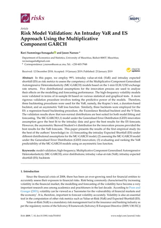
The figure below (Figure 6) displays the volatility decomposition into the different components
for the MC-GARCH model under GED innovation: the diurnal component, the daily volatility
component, the intradaily volatility component, and the total composite volatility for the intraday 1-
min data, which is obtained by combining the three volatility components.
Figure 5. Empirical density of the standardised residuals.
The figure below (Figure 6) displays the volatility decomposition into the different components for
the MC-GARCH model under GED innovation: the diurnal component, the daily volatility component,

Risks 2019, 7, 10 15 of 23
the intradaily volatility component, and the total composite volatility for the intraday 1-min data,
which is obtained by combining the three volatility components.
Figure 6. Diurnal component, daily volatility component, intradaily volatility component, and total
composite volatility.
The MC-GARCH model is also valid, since it includes a component to cater for the intraday
seasonality (sigma (Diurnal)).
4.7. Intraday VaR Forecast
The 99% intraday VaR is forecasted using the MC-GARCH models on the 1-min intraday return
series. A rolling backtest procedure is then undertaken on the out-sample period and a moving
window of 1 day will be used in the VaR backtesting procedure. The backtesting period is one day,
which relates to 1500 1-min datapoints.
4.7.1. Kupiec’s Test
The first backtest used is the Kupiec’s unconditional coverage test, where the 1500 intraday VaR
forecasts estimated are compared against the actual intraday returns. The results (Table 5) of the
backtest speaks in favour of the MC-GARCH model, as all the models, except the MC-GARCH under
the normal distribution, passed this test since the p-values, being greater than the 5% significance
level, indicate that the null hypothesis cannot be rejected.
Table 5. Intraday VaR forecast: Kupiec’s test.
Expected VaR Exceedances 15 15 15 15 15
Actual VaR Exceedances 27 21 22 21 20
Actual % 1.80% 1.40% 1.50% 1.40% 1.30%
p-value 0.005 0.142 0.089 0.142 0.217
Figure 6. Diurnal component, daily volatility component, intradaily volatility component, and total
composite volatility.
The MC-GARCH model is also valid, since it includes a component to cater for the intraday
seasonality (sigma (Diurnal)).
4.7. Intraday VaR Forecast
The 99% intraday VaR is forecasted using the MC-GARCH models on the 1-min intraday return
series. A rolling backtest procedure is then undertaken on the out-sample period and a moving
window of 1 day will be used in the VaR backtesting procedure. The backtesting period is one day,
which relates to 1500 1-min datapoints.
4.7.1. Kupiec’s Test
The first backtest used is the Kupiec’s unconditional coverage test, where the 1500 intraday VaR
forecasts estimated are compared against the actual intraday returns. The results (Table 5) of the
backtest speaks in favour of the MC-GARCH model, as all the models, except the MC-GARCH under
the normal distribution, passed this test since the p-values, being greater than the 5% significance level,
indicate that the null hypothesis cannot be rejected.
Table 5. Intraday VaR forecast: Kupiec’s test.
Expected VaR
Exceedances
15 15 15 15 15
Actual VaR Exceedances 27 21 22 21 20
Actual % 1.80% 1.40% 1.50% 1.40% 1.30%
p-value 0.005 0.142 0.089 0.142 0.217

Risks 2019, 7, 10 16 of 23
4.7.2. VaR Duration Test
The results of the VaR duration test are displayed in Table 6.
Table 6. Intraday VaR forecast: duration-based approach VaR backtesting results.
Model b p-Value
MC-GARCH_norm 0.877439 0.397975
MC-GARCH_std 0.85151 0.392917
MC-GARCH_sstd 0.85151 0.392917
MC-GARCH_jsu 0.85151 0.392917
MC-GARCH_ged 0.85151 0.392917
The second column ‘b’ is the estimated Weibull parameter for the different models. Since the
p-values for all models are greater than the significance level of 5%, this gives evidence that the
duration of time between the VaR violations possess no memory and that they do not cluster. All the
models passed the VaR duration-based backtest.
4.7.3. Backtesting VaR Using an Asymmetric Loss Function
A more rigorous backtesting procedure is carried out. As stated in Bernardi et al. (2014), though
the Kupiec’s test is able to compare VaR violations of several competing models, it fails, however, to
rank the models according to their predictive accuracy of the VaRs. Moreover, many models satisfy the
unconditional coverage test, as it is observed in this study. The risk manager therefore cannot select
a unique method. Lopez (1998) suggested to measure the accuracy of VaR forecasts based on a loss
function and the models are ranked accordingly.
To present results which are less sensitive to the low number of theoretical violations and to
deal with the problem of the Kupiec’s test, the Model Confidence Set (MCS) procedure proposed by
Hansen et al. (2011) is applied together with the asymmetric VaR function of González-Rivera et al.
(2004). The results for the MCS procedure are presented in Table 7. Only those models which passed
the Kupiec’s test and the VaR duration test are considered. The best-performing model according to
this procedure is the MC-GARCH under the skewed Student’s-t distribution, since it minimises the
loss function.
Table 7. Intraday VaR forecast: MCS results and ranking.
Superior Set of Model
Model Rank Loss (× 10−6)
MC-GARCH_std 2 4.61995
MC-GARCH_sstd 1 4.615442
MC-GARCH_jsu 4 4.744222
MC-GARCH_ged 3 4.639826
The sigma forecast plot and the VaR backtesting plot for the MC-GARCH(1,1) model under the
skewed Student’s-t distribution are displayed below in Figures 7 and 8 respectively.

Risks 2019, 7, 10 17 of 23
Figure 7. Sigma forecast plot.
As noted in Singh et al. (2013), the spikes in the VaR forecasts as shown in the backtest plot in
Figure 8 is due to the seasonal component during the opening of each trading day.
Figure 8. VaR backtest graph.
4.8. Intraday ES Forecast
The backtesting of the Expected Shortfall (ES) is now conducted, and three backtests are
implemented to determine the accuracy of the ES forecast.
4.8.1. A Regression-Based ES Backtesting Procedure: the Bivariate ES Regression Backtest
The results for this backtest, both with and without bootstrapping, are shown in Table 8, below.
All p-values are greater than the 5% significance level. The null hypothesis, which states that the ’ES
forecasts are correctly specified’ is not rejected. Moreover, the bootstrap p-values are also highly
significant. Therefore, it can be concluded that the MC-GARCH models are able to forecast accurately
the risk measure ES.
Table 8. Intraday ES forecast: bivariate ESR backtest results.
Model p-Value Boot p-Value
MC-GARCH_std 0.806 0.580
MC-GARCH_sstd 0.763 0.527
MC-GARCH_jsu 0.755 0.492
MC-GARCH_ged 0.868 0.664
Two classical ES backtests are employed to determine which model delivers the best ES
estimates.
All p-values are greater than the 5% significance level. The null hypothesis, which states that the ’ES
forecasts are correctly specified’ is not rejected. Moreover, the bootstrap p-values are also highly
Two classical ES backtests are employed to determine which model delivers the best ES
estimates.
All p-values are greater than the 5% significance level. The null hypothesis, which states that the
’ES forecasts are correctly specified’ is not rejected. Moreover, the bootstrap p-values are also highly
Two classical ES backtests are employed to determine which model delivers the best ES estimates.

Risks 2019, 7, 10 18 of 23
4.8.2. Exceedance Residual (ER) Backtest
The Exceedance Residual (ER) backtest of McNeil and Frey (2000) is also employed in this paper.
The corresponding results are displayed in Table 9, below.
Table 9. Intraday ES forecast: Exceedance Residual (ER) backtest.
Model Expected Exceedances Actual Exceedances p-Value
MC-GARCH_std 15 21 0.1845
MC-GARCH_sstd 15 22 0.1322
MC-GARCH_jsu 15 21 0.1302
MC-GARCH_ged 15 20 0.1077
The null hypothesis, which states that “Mean of Excess Violations of VaR is Equal to zero”, is not
rejected, since all p-values are greater than 5% confidence level. Based on this backtesting procedure,
it can therefore be ascertained that the MC-GARCH models succeed in accurately predicting the
ES estimates. Although the actual ES exceedances are comparable across the four MC-GARCH
specifications, it can be observed that the MC-GARCH model under the GED error ditribution yields
the least exceedances.
4.8.3. V-Tests
The V-Test statistics backtesting procedure can be regarded more as a diagnostic tool than a formal
statistical testing procedure, since there is no null hypothesis involved.
Table 10 displays the results for the V1, V2 and V3 test statistics. The first observation is that
the sign of the V1, V2 and V3 test statistics are positive, thus implying that all the models are, on
average, overestimating the ES risk measure. Moreover, since the magnitude of the values of the test
statistics are very close to zero, it implies that the models are only slightly overestimating the ES.
These results speak in favour of the MC-GARCH models since risk managers are less concerned about
overestimation of the risk metric as compared to an underestimation.
Table 10. Intraday ES Forecast: V-tests Backtesting Results.
Model V1 V2 V
MC-GARCH_std 0.0004419 0.0015778 0.0010099
MC-GARCH_sstd 0.0004391 0.0015690 0.0010041
MC-GARCH_jsu 0.0004383 0.0015667 0.0010025
MC-GARCH_ged 0.0004243 0.0015206 0.0009724
Furthermore, it can be observed that the magnitude of the V1 test statistic is smaller for
the MC-GARCH model under GED innovation assumption as compared to the other innovation
assumptions thereby indicating that it performs relatively better. The same observation can be made
for the other two test statistics, V2 and V3. Therefore, the MC-GARCH model under the GED error
ditribution is the best model for ES under this backtest.
Figure 9 displays the ES forecasts for the MC-GARCH model under the GED innovation process.
Once more it can be seen that the MC-GARCH models are able to adequately forecast ES.

Risks 2019, 7, 10 19 of 23
Figure 9. ES backtest graph for MC-GARCH_GED.
Figure 10 displays the forecast for both VaR and ES at 99% for the MC-GARCH_GED model.
Figure 10. Backtest graph for MC-GARCH_GED.
5. Conclusions
A typical question that sparks a lot of interest in the high-frequency trading literature concerns
which GARCH model tends to be the best when it comes to forecasting intradaily risk metrics such
as Value-at-Risk (VaR) and Expected Shortfall (ES). This paper therefore focuses on the performance
analysis of the MC-GARCH model in forecasting 1-min VaR and 1-min ES.
The first objective of this study was to determine which GARCH-type model gives the best in-
sample fit to the daily EUR/USD returns for the daily variance forecast for the MC-GARCH model. It
was found that overall the EGARCH(1,1) models were preferred over the GARCH(1,1) models. The
EGARCH model under the GED innovation assumption however yielded the best results.
The second aim of the study was to analyse the effects of different distributional assumption for
the innovation process of the GARCH models for both model fitting and forecasting. Overall, it was
5. Conclusions
The first objective of this study was to determine which GARCH-type model gives the best in-
sample fit to the daily EUR/USD returns for the daily variance forecast for the MC-GARCH model. It
was found that overall the EGARCH(1,1) models were preferred over the GARCH(1,1) models. The
EGARCH model under the GED innovation assumption however yielded the best results.
The second aim of the study was to analyse the effects of different distributional assumption for
the innovation process of the GARCH models for both model fitting and forecasting. Overall, it was
5. Conclusions
The first objective of this study was to determine which GARCH-type model gives the best
in-sample fit to the daily EUR/USD returns for the daily variance forecast for the MC-GARCH model.
It was found that overall the EGARCH(1,1) models were preferred over the GARCH(1,1) models.
The EGARCH model under the GED innovation assumption however yielded the best results.
The second aim of the study was to analyse the effects of different distributional assumption
for the innovation process of the GARCH models for both model fitting and forecasting. Overall, it
was found that non-normal distributional assumptions gave better results for model fitting as well as

Risks 2019, 7, 10 20 of 23
forecasting. This is due to the fact that non-normal distributions are able to take into account features
such as excess kurtosis and asymmetry of the high-frequency EUR/USD returns. Furthermore, they
are able to replicate these features when forecasting volatility. The MC-GARCH(1,1) model under the
GED innovation assumption actually gave the best fit to the intraday data as per the ranking procedure
carried out based on AIC, BIC and log-likelihood criteria.
The one-day ahead 99% intraday VaR values were forecasted using the MC-GARCH models.
Three VaR backtesting procedures were carried out namely the Kupiec’s test, the VaR duration-based
backtest and a backtest based on an asymmetric VaR loss function. Based on the number of VaR
violations, the MC-GARCH(1,1) model under the GED distribution gave the best results. When the
asymmetric VaR loss function, which is a more robust backtesting procedure, was implemented, the
MC-GARCH(1,1) model under the skewed Student’s-t distribution minimised the loss function with
the smallest value and proved to be the best model.
The one-day ahead 99% intraday ES was also forecasted using these models. Three backtesting
procedures were employed for the ES, namely, the Bivariate ES regression backtest, the Exceedance
Residuals backtest and the V-tests. It was found that the MC-GARCH models under the non-normal
distribution assumptions are able to produce accurate intraday ES forecasts. The MC-GARCH(1,1)
model under the GED distribution however yields the best results.
5.1. Recommendations for Practitioners
It is recommended to avoid the use of normal innovation distribution for MC-GARCH modelling,
as it significantly overestimates risk. Such risk overestimation in the insurance and banking industries
may actually lead to an excess of capital requirements, which may be unnecessary and hence
loss-making for the institution. The MC-GARCH, under other innovation distributions such as
Student’s-t, the Skewed Student’s-t distribution (sstd), the reparametrised Johnson SU (JSU) and the
Generalised Error Distribution (GED), also overestimates the risk metrics, but yields empirical sizes
closer to the expected size for both the VaR and ES. It is, however, recommended to employ the
MC-GARCH(1,1) model under the GED distribution as it yields least overestimation results, which
minimise the excess of capital requirement.
5.2. Further Studies
There still exist a multitude of areas for further research using the MC-GARCH models. Other
distributional assumptions for the innovation process such as the skewed GED, Normal Inverse
Gaussian (NIG) can be implemented. Moreover, the performance of the MC-GARCH models in
predicting the risk metrics VaR and ES at higher confidence levels such as 99.5% or even 99.9% can
also be assessed. The combination of Extreme Value Theory (EVT) with the MC-GARCH model can be
analysed in forecasting intraday VaR and ES. A comparison between the MC-GARCH-EVT and the
MC-GARCH models in predicting VaR and ES at different sampling frequency such as 1-min, 5-min
and 10 min returns would be a particularly interesting study.
Author Contributions: Conceptualization, J.N.; Formal analysis, R.S.S.; Methodology, R.S.S. and J.N.; Software,
R.S.S.; Supervision, J.N.; Validation, R.S.S.; Writing—original draft, R.S.S.; Writing—review editing, J.N.
Funding: This research received no external funding.
Acknowledgments: The authors thank the reviewers for their valuable suggestions.
Conflicts of Interest: The authors declare no conflict of interest.
Appendix A
The preliminary analysis is laid out in this section.
It can be seen in Table A1 that the mean for both series hovers around 0 which in fact coincides
with past studies on high-frequency financial returns. Moreover, the skewness values for both return
series are negative which may imply that these series experience more negative shocks than positive

Risks 2019, 7, 10 21 of 23
shocks and that there is a higher probability of obtaining a negative return. All kurtosis values
being greater than 3, which is the kurtosis of any univariate normal distribution, imply that return
distributions have thicker tails and sharper peaks at the centre as compared to a normal distribution.
When comparing the degree of kurtosis and skewness for the 1-min returns (18.31108, −0.38839) with
that of the daily returns (4.90965, −0.08208), it can be established that the kurtosis and the skewness
values are much higher for the 1-min returns. This suggests that both the kurtosis and the degree of
skewness increase with the frequency at which the data is recorded, thus confirming the findings of
Andersen and Bollerslev (1998). The high kurtosis value for the 1-min returns is yet another stylised
fact of high-frequency financial returns. The minimum value for the daily return occurred during the
global financial crisis.
Table A1. EUR/USD Returns descriptive statistics.
1-min Returns Daily Returns
Mean 1.23 × 10−7 4.62 × 10−5
Standard deviation 0.00017 0.00633
Maximum 0.00193 0.02781
Minimum −0.00332 −0.03733
Skewness −0.38839 −0.08208
Kurtosis 18.31108 4.90965
Observations 28,289 3159
These will aid to further confirm the presence of different stylised facts present in the return series.
To further demonstrate that both returns series deviate from normality, the Jarque-Bera (JB) test
is carried out and their kernel estimates of the density are inspected. The results are presented in
Table A2.
Table A2. Jarque Bera test.
Test Statistic p-Value Decision
1-min returns 277,030 0 Reject H0
Daily returns 483.55 0 Reject H0
The p-value for the 1-min returns and for the daily returns series being equal to 0 for the JB
normality test allows us to safely conclude, at a 5% significance level, that indeed these distributions
do not follow a normal distribution. The same conclusion can be derived when analyzing the kernel
density estimates in Figure A1 for both the 1 min returns (left) and the daily returns (right) since they
clearly display leptokurticity.
To determine whether the series is stationary, the Augmented Dickey-Fuller (ADF) test is carried
out on both return series. If the ADF test detects the presence of a unit root in the series, it can be
deduced that the series is non-stationary and need differencing. Table A3 shows the results for the
ADF test:
Table A3. ADF test.
Test Statistic Lag Order p-Value
1-min returns −30.596 30 0.01
Daily returns −14.03 14 0.01

Risks 2019, 7, 10 22 of 23
Figure A1. Kernel density estimates for 1 min returns (left) and daily returns (right).
The p-values for both returns series are less than 5% and this allows the rejection of the null
hypothesis that a unit root is present in the series. Therefore, both return series are stationary and the
order of the parameter 𝑑 in the ARIMA(𝑝, 𝑑, 𝑞) model for both series is equal to 0.
References
(Andersen and Bollerslev 1997) Andersen, Torben G., and Tim Bollerslev. 1997. Intraday periodicity and
volatility persistence in financial markets. Journal of Empirical Finance 4: 115–58. doi:10.1016/s0927-
5398(97)00004-2.
(Andersen and Bollerslev 1998) Andersen, Torben G., and Tim Bollerslev. 1998. Answering the Skeptics: Yes,
Standard Volatility Models do Provide Accurate Forecasts. International Economic Review 39: 885.
doi:10.2307/2527343.
(Andersen et al. 1999) Andersen, Torben G., Tim Bollerslev, and Steve Lange. 1999. Forecasting financial market
volatility: Sample frequency vis-à-vis forecast horizon. Journal of Empirical Finance 6: 457–77.
doi:10.1016/s0927-5398(99)00013-4.
(Bayer and Dimitriadis 2018) Bayer, Sebastian, and Timo Dimitriadis. 2018. Regression Based Expected Shortfall
Backtesting. arXiv. arXiv:1801.04112.
(BCBS 2010) Basel Committee on Banking Supervision. 2010. Basel III: A Global Regulatory Framework for More
Resilient Banks and Banking Systems. Basel: Bank for International Settlements.
(BCBS 2012) Basel Committee on Banking Supervision. 2012. Fundamental Review of the Trading Book. Basel: Bank
for International Settlements.
(BCBS 2016) Basel Committee on Banking Supervision. 2016. Minimum Capital Requirements for Market Risk. Basel:
Bank for International Settlements.
(Bernardi et al. 2014) Bernardi, Mauro, Leopoldo Catania, and Lea Petrella. 2014. Are news important to predict
large losses? arXiv. arXiv:1410.6898.
(Bollerslev 1987) Bollerslev, Tim. 1987. A Conditionally Heteroskedastic Time Series Model for Speculative
Prices and Rates of Return. The Review of Economics and Statistics 69: 542. doi:10.2307/1925546.
(Christoffersen and Pelletier 2003) Christoffersen, Peter, and Denis Pelletier. 2003. Backtesting Value-at-Risk: A
Duration-Based Approach. SSRN Electronic Journal. doi:10.2139/ssrn.418762.
(Culp et al. 1998) Culp, Christopher L., Merton H. Miller, and Andrea MP Neves. 1998. Value at Risk: Uses and
Abuses. Journal of Applied Corporate Finance 10: 26–38.
Figure A1. Kernel density estimates for 1 min returns (left) and daily returns (right).
The p-values for both returns series are less than 5% and this allows the rejection of the null
hypothesis that a unit root is present in the series. Therefore, both return series are stationary and the
order of the parameter d in the ARIMA(p, d, q) model for both series is equal to 0.
References
Andersen, Torben G., and Tim Bollerslev. 1997. Intraday periodicity and volatility persistence in financial markets.
Journal of Empirical Finance 4: 115–58. [CrossRef]
Andersen, Torben G., and Tim Bollerslev. 1998. Answering the Skeptics: Yes, Standard Volatility Models do
Provide Accurate Forecasts. International Economic Review 39: 885. [CrossRef]
Andersen, Torben G., Tim Bollerslev, and Steve Lange. 1999. Forecasting financial market volatility: Sample
frequency vis-à-vis forecast horizon. Journal of Empirical Finance 6: 457–77. [CrossRef]
Bayer, Sebastian, and Timo Dimitriadis. 2018. Regression Based Expected Shortfall Backtesting. arXiv,
arXiv:1801.04112.
Basel Committee on Banking Supervision. 2010. Basel III: A Global Regulatory Framework for More Resilient Banks
and Banking Systems. Basel: Bank for International Settlements.
Basel Committee on Banking Supervision. 2012. Fundamental Review of the Trading Book. Basel: Bank for
International Settlements.
Basel Committee on Banking Supervision. 2016. Minimum Capital Requirements for Market Risk. Basel: Bank for
International Settlements.
Bernardi, Mauro, Leopoldo Catania, and Lea Petrella. 2014. Are news important to predict large losses? arXiv,
arXiv:1410.6898.
Bollerslev, Tim. 1987. A Conditionally Heteroskedastic Time Series Model for Speculative Prices and Rates of
Return. The Review of Economics and Statistics 69: 542. [CrossRef]
Christoffersen, Peter, and Denis Pelletier. 2003. Backtesting Value-at-Risk: A Duration-Based Approach. SSRN
Electronic Journal. [CrossRef]
Culp, Christopher L., Merton H. Miller, and Andrea M. P. Neves. 1998. Value at Risk: Uses and Abuses. Journal of
Applied Corporate Finance 10: 26–38. [CrossRef]
Diao, Xundi, and Bin Tong. 2015. Forecasting intraday volatility and VaR using multiplicative component GARCH
model. Applied Economics Letters 22: 1457–64. [CrossRef]
Efron, Bradley, and Robert J. Tibshirani. 1994. An Introduction to the Bootstrap. Boca Raton: Chapman Hall/CRC.
Engle, Robert F. 1982. A general approach to lagrange multiplier model diagnostics. Journal of Econometrics 20:
83–104. [CrossRef]

Risks 2019, 7, 10 23 of 23
Engle, Robert Fry, and Jeffrey Russell. 2004. Analysis of High Frequency Financial Data. In Handbook of Financial
Econometrics. Edited by Yacine Ait-Sahalia and Lars Hansen. Amsterdam: North Holland Press.
Engle, Robert F., and Magdalena E. Sokalska. 2011. Forecasting intraday volatility in the US equity market.
Multiplicative component GARCH. Journal of Financial Econometrics 10: 54–83. [CrossRef]
García Jorcano, Laura. 2018. Sample Size, Skewness and Leverage Effects in Value at Risk and Expected Shortfall
Estimation. Ph.D. Dissertation, Universidad Complutense de Madrid, Madrid, Spain.
Giot, Pierre. 2000. Time transformations, intraday data, and volatility models. The Journal of Computational Finance
4: 31–62. [CrossRef]
González-Rivera, Gloria, Tae-Hwy Lee, and Santosh Mishra. 2004. Forecasting volatility: A reality check based on
option pricing, utility function, value-at-risk, and predictive likelihood. International Journal of Forecasting 20:
629–45. [CrossRef]
Hansen, Peter R., Asger Lunde, and James M. Nason. 2011. The Model Confidence Set. Econometrica 79: 453–97.
[CrossRef]
Kupiec, Paul. 1995. Techniques for Verifying the Accuracy of Risk Measurement Models. The Journal of Derivatives
3: 73–84. [CrossRef]
Lopez, Jose A. 1998. Methods for Evaluating Value-at-Risk Estimates. SSRN Electronic Journal. [CrossRef]
McNeil, Alexander J., and Rüdiger Frey. 2000. Estimation of tail-related risk measures for heteroscedastic financial
time series: An extreme value approach. Journal of Empirical Finance 7: 271–300. [CrossRef]
McNeil, Alexander J., Rüdiger Frey, and Paul Embrechts. 2005. Quantitative Risk Management: Concepts, Techniques
and Tools. Princeton: Princeton University Press.
Mondal, Prapanna, Labani Shit, and Saptarsi Goswami. 2014. Study of Effectiveness of Time Series Modeling
(Arima) in Forecasting Stock Prices. International Journal of Computer Science, Engineering and Applications 4:
13–29. [CrossRef]
Müller, Ulrich A. 2000. Volatility Computed by Time Series Operators at High Frequency. SSRN Electronic Journal.
[CrossRef]
Narsoo, Jason. 2016. High Frequency Exchange Rate Volatility Modelling Using the Multiplicative Component
GARCH. International Journal of Statistics and Applications 6: 8–14.
Nelson, Daniel B. 1991. Conditional Heteroskedasticity in Asset Returns: A New Approach. Econometrica 59: 347.
[CrossRef]
Poon, Ser-Huang, and C. Granger. 2001. Forecasting Financial Market Volatility: A Review. SSRN Electronic
Journal. [CrossRef]
Singh, Abhay Kumar, David E. Allen, and Robert J. Powell. 2013. Intraday Volatility Forecast in Australian Equity
Market. SSRN Electronic Journal. [CrossRef]
Tsay, Ruey S. 2005. Analysis of Financial Time Series. New York: Wiley.
Zivot, Eric. 2005. Analysis of High Frequency Financial Data: Models, Methods and Software. Part I: Descriptive
Analysis of High Frequency Financial Data with S-PLUS. Available online: https://faculty.washington.edu/
ezivot/research/hflectures.pdf (accessed on 15 January 2019).
© 2019 by the authors. Licensee MDPI, Basel, Switzerland. This article is an open access
article distributed under the terms and conditions of the Creative Commons Attribution
(CC BY) license (http://creativecommons.org/licenses/by/4.0/).

risks-07-00010-v3 (1).pdf

Recommended

Recommended

More Related Content

Similar to risks-07-00010-v3 (1).pdf

Similar to risks-07-00010-v3 (1).pdf (20)

Recently uploaded

Recently uploaded (20)

risks-07-00010-v3 (1).pdf