Beyond Broken Stick Modeling: R Tutorial for interpretable multivariate analysis

Petteri Teikari
MSc Electrical Engineering
PhD, Neuroscience
http://petteri-teikari.com/
Singapore Eye Research Institute (SERI)
Visual Neurosciences group
version Tue 28 August 2018
Beyond
BROKEN STICK
“R Tutorial” for Interpretable
multivariate analysis with t-
SNE and Random Forests, etc.
http://doi.org/10.1098/rsif.2014.0672
https://youtu.be/nS1X5OEulDY
https://doi.org/10.1016/j.jbi.2017.10.006

Broken Stick Model
Bruch s membrane opening-minimum rim width and visual field'
loss in glaucoma: a broken stick analysis
https://dx.doi.org/10.18240%2Fijo.2018.05.19
Measurement of macular structure-function relationships using
spectral domain-optical coherence tomography (SD-OCT) and
pattern electroretinograms (PERG).
http://dx.plos.org/10.1371/journal.pone.0178004
“The normal”
region
Still appear
normal, “False Negative”
“Glaucomatous”
patients, “True Positive”
Point wherethe
“stickbreaks”
Scatter plots showing relationship of central visual field sensitivities (A, B, C) or
visual field mean deviation (D, E, F) with ganglion cell/inner plexiform layer
(GCIPL) thickness

Broken Stick i.e.segmentedregressionworksforsomedata
http://jeb.biologists.org/content/205/24/3945
Package segmented - CRAN.R-project.org' '
by VMR Muggeo - 2017 - Cited by 17 - Related articles
https://youtu.be/onfXC1qe7LI
How to Develop a Piecewise Linear Regression Model in R
Shokoufeh Mirzaei
Published on Jan 28, 2018
Not themost powerfultechnique though
for nonlinear interactions as you can assume

Dataset do we have “all the relevant” features

You also want to know whether given measure for the
given patient is reliable
https://www.eyeworld.org/don-t-be-fooled-artifacts-retinal-nerve-fiber-layer-oct
Quality assessment for spectral domain optical coherence tomography
(OCT) images
https://arxiv.org/abs/1703.04977
Iftheimage qualityis bad, the derived
OCTmeasurements have increased
uncertainty as well

Artifacts might tell you something about the disease as well
Prevalencesof segmentationerrorsandmotionartifactsinOCT-angiography diferamongretinaldiseases
J.L.Lauermann,A.K.Woetzel,M.Treder,M.Alnawaiseh,C.R.Clemens,N. Eter,FlorianAlten
Graefe'sArchiveforClinicalandExperimentalOphthalmology(07July2018)
https://doi.org/10.1007/s00417-018-4053-2
Spectral domain OCT-A device (Optovue Angiovue) showing diferent degrees of motion artifacts.
a Motion artifact score (MAS) b, c Manifestation of diferent motion artifacts, including strong
quilting, partly with incipient expression of black lining (white asterisk), stretching (white arrows),
and displacements(whitecircles) in diferent partsof theimage
In the future, deep learning software applications might not only be able to distinguish between different retinal diseases but also to detect
specific artifacts and to warn the user in case of insufficient image quality. Today, multimodal imaging leads to an overwhelmingly large amount
of image information that has to be reviewed by ophthalmologists in daily clinical routine. Thus, software assistance in image grading appears
mandatory to manage the growing amount of image data and to avoid useless image data of insufficient quality. In the future, segmentation
will move forward through redefinitions of segmentation boundaries and refinements of algorithm strategies in pathologic maculae [
de Sisternes et al. 2017]. In conclusion, OCT-A image quality including motion artifacts and segmentation errors must be assessed prior to a
detailed qualitative or quantitative analysis to warrant meaningful and reliable results.

Myopia and RNFL thickness and image quality?
Qiu et al. 2018:
“Thisstudyaimedtodetermine the infuence ofthe
opticdisc-foveadistance(DFD) on macular
thicknessinmyopiceyes.... Ourfndingsindicate
that eyeswithagreaterDFD have alowermacular
thickness.”,
“It has been reported that the image quality ofOCT scans
afects theobserved retinal layer thicknesses [
Huang et al. 2011; Darmaet al. 2015; Jansonius et al. 2016],
andimagequality decreaseswith anincreasein
myopia[Lee et al. 2018].”
Zhaetal.2017
Inconclusion,myopiadidhave
specialinfuenceonRNFL
thickness, whichwasnot related
tosexor age.
Withthe nice“diurnalprofle”
https://doi.org/10.3341/jkos.2009.50.12.1840

Evaluation of a
Myopic Normative
Database for
Analysis of
Retinal Nerve
Fiber Layer
Thickness
http://doi.org/10.1001/jamaophth
almol.2016.2343

Clinical modelling often not very linear though
High-level motivation to go beyond the Broken Stick

Multivariate Examples 1#
Dynamic Modeling of Multivariate Latent Processes and Their
Temporal Relationships: Application to Alzheimer s Disease'
Bachirou O. Taddé, Hélène Jacqmin-Gadda, Jean-FrançoisDartigues, Daniel Commenges, Cécile
Proust-Lima| NSERM, UMR1219, Univ. Bordeaux,
Alzheimer's disease gradually afects several componentsincluding
the cerebral dimension with brain atrophies, the cognitive dimension
with a decline in various functions and the functional dimension with
impairment in the daily living activities. Understanding how such
dimensions interconnect is crucial for AD research. However it requires
to simultaneously capture the dynamic and multidimensional
aspects, and to explore temporal relationships between
dimensions. We propose an original dynamic model that accounts for
all these features. The model defnes dimensions as latent
processes and combines a multivariate linear mixed model and a
system of diference equations to model trajectories and temporal
relationshipsbetween latentprocessesin fnelydiscrete time.
We demonstrate in a simulation study that this dynamic
model in discrete time benefts the same causal
interpretation of temporal relationships as
mechanistic models defned in continuous time.

Nonlinear Multivariate Examples 1#
Multivariate joint frailty model for the analysis of nonlinear tumor
kinetics and dynamic predictions of death
StatisticsinMedicine Volume37, Issue1315June 2018 Pages2148-2161
AgnieszkaKról etal. (2018)
https://doi.org/10.1002/sim.7640
Usually, a biomarker is analyzed with a linear mixed model; more fexible
trajectory can be obtained using diferent forms of the parametric approach.
The longitudinal trajectory of a biomarker can also be approximated using
splines, eg, B-splines. More fexible and sophisticated analyses are provided
by approaches that assume mechanistic models for biomarker dynamics.
These models could provide more accurate modeling of the biological
process and account at the same time for the heterogeneity in the data
andprognosticfactors.
Here, we propose a multivariate joint frailty model for longitudinal data
represented by a solution to ordinary diferential equations (ODE), recurrent
events, and a terminal event. We perform a simulation study in which we
compare this model to a joint model with a 2-phase linear mixed-efects
model for the sumofthe longestdiameters(SLD) andtoajointmodelapplying
B-splines for the SLD trajectory in terms of goodness of ft and predictive
accuracy.
All the models were estimated using the extensions of the R package frailtypack
(https://www.jstatsoft.org/article/view/v081i03) The mechanistic joint frailty model
that uses the analytical solution to the ODE
Estimating nonlinear effects in the presence of cure fraction using
a semi-parametric regression model
ComputationalStatisticsJune 2018, Volume33, Issue 2, pp 709–730
ThiagoG. Ramiresetal. (2017)
https://doi.org/10.1007/s00180-017-0781-8
The proposed model isbased on the generalized additive models (GAMs)
for location, scale and shape, for which any or all parameters of the distribution
are parametric linear and/or nonparametric smooth functions of explanatory
variables. The new model is used to ft the nonlinear behavior between
explanatory variables and cure rate. The biases of the cure rate
parameter estimates caused by not incorporating such non-linear efects in the
model are investigated using Monte Carlo simulations. We discuss diagnostic
measures and methods to select additive terms and their computational
implementation
Codes implemented in the GAMLSS package in the software R

Data adaptive additive modeling‐
StatisticsinMedicine https://doi.org/10.1002/sim.7859
AshleyPetersen and DanielaWitten (2018)
For instance, the sparse additive model makes it
possible to adaptively determine which features
should be included in the ftted model, the sparse
partially linear additive model allows each feature in
the ftted model to take either a linear or a
nonlinear functional form, and the recent fused
lasso additive model and additive trend fltering
proposals allow the knots in each nonlinear function ft
tobe selectedfromthedata.
Inthispaper,wecombinethestrengthsofeachofthese
recent proposals into a single proposal that uses the
data to determine which features to include in the
model, whether to model each feature linearly
or nonlinearly, and what form to use for the
nonlinearfunctions.
Modeling decisions required when fitting an additive model of the
form in Equation 1. We seek to develop an estimator that can make
all three decisions in a data-adaptive way

Estimating individualized optimal
combination therapies through outcome
weighted deep learning algorithms
https://tensorfow.rstudio.com/ Keras/ Tensorfowin R
MuxuanLiang, TingYe, HaodaFu(2018)
With the advancement in drug development, multiple treatments are
available for a single disease. Patients can often beneft from taking
multiple treatments simultaneously. For example, patients in
Clinical Practice Research Datalink with chronic diseases such as
type 2 diabetes can receive multiple treatments simultaneously.
Therefore, it is important to estimate what combination
therapy from which patients can beneft the most. However, to
recommend the best treatment combination is not a single label but
a multilabel classifcation problem. In this paper, we propose a
novel outcome weighted deep learning algorithm to estimate
individualizedoptimalcombinationtherapy.
The Fisher consistency of the proposed loss function under certain
conditions is also provided. In addition, we extend our method to a
family of loss functions, which allows adaptive changes based on
treatment interactions. We demonstrate the performance of our
methodsthrough simulationsandrealdataanalysis.

Personalized Risk Prediction in Clinical
Oncology Research: Applications and
Practical Issues Using Survival Trees
and Random Forests
Chen Hu & Jon ArniSteingrimsson
Journal ofBiopharmaceuticalStatistics
Volume28,2018- Issue2:SpecialIssue:Precision Medicinein CancerResearch
https://doi.org/10.1080/10543406.2017.1377730
Risk prediction models used in clinical oncology commonly use both
traditional demographic and tumor pathological factors as well as
high-dimensional genetic markers and treatment parameters from
multimodality treatments. In this article, we describe the most
commonly used extensions of the Classifcation and
Regression Tree (CART) and random forest algorithms to right-
censoredoutcomes.
We focus on how they difer from the methods for noncensored
outcomes, and how the diferent splitting rulesand methodsfor cost-
complexity pruning impact these algorithms. These simulation
studies aim to evaluate how sensitive the prediction accuracy is to
the underlying model specifcations, the choice of tuning
parameters,andthedegreesofmissingcovariates.

Utilization of Low Dimensional Structure to
Improve the Performance of
Nonparametric Estimation in High
Dimensions
eScholarship -UCLA - UCLA Electronic Theses and Dissertations
Conn, Daniel Joshua
https://escholarship.org/uc/item/9z03w0zk
First, we have developed a variant of random forests, called fuzzy forests. Fuzzy
forests reduce the bias observed in random forest variable importance measures by
clustering covariates into distinct groupssuch that the correlation ofcovariateswithin a
group is high and the correlation between groups is low. Fuzzy forests is expected to
workwellwhen thetrueregressionfunctionexhibitsan additivestructure.
Flow chart of fuzzy forests algorithm

Visualize for clinicians with uncertainty

Random Forest VIMP the easiest route
https://dinsdalelab.sdsu.edu/metag.stats/code/randomforest.html
library(randomForest)
https://www.biostars.org/p/86981/
Tutorial: Machine Learning For Cancer
Classification
library(randomForest)
library(ROCR)
library(genefilter)
library(Hmisc)

Variable Importance 1#
Correlation and variable importance in
random forests
StatisticsandComputingMay2017,Volume27,Issue3,pp659–678
https://doi.org/10.1007/s11222-016-9646-1
Baptiste Gregorutti, Bertrand Michel, Philippe Saint-Pierre
Our results motivate the use of the recursive
feature elimination (RFE) algorithm for variable
selection in this context. This algorithm
recursively eliminates the variables using
permutation importance measure as a ranking
criterion. Next various simulation experiments
illustrate the efciency of the RFE algorithm for
selecting a small number of variables
together with agoodprediction error.
In future works, the algorithm could be adapted by
combining a non recursive strategy at the frst
steps and a recursive strategy at the end of the
algorithm.
Boxplots of the initial permutation
importance measures. In each group,
only the ten variables with the
highest importances are displayed
Boxplots of the initial permutation importance
measures. For each group, only the predictive
variable (dashed lines) and the two variables
with the highest importance in the same group
(solid lines) are displayed

Standard errors and confidence
intervals for variable importance in
random forest regression, classification,
and survival
Hemant Ishwaran and Min Lu(2018)
Random forests are a popular nonparametric tree
ensemble procedure with broad applications to data
analysis. While its widespread popularity stems from
its prediction performance,anequally importantfeature
is that it provides a fully nonparametric measure of
variableimportance(VIMP)
We propose a subsampling approach that can be
used to estimate the variance of VIMP and for
constructing confdence intervals. Using extensive
simulations, we demonstrate the efectiveness of the
subsampling estimator and in particular fnd that the
delete d jackknife variance estimator‐ , a close
cousin, is especially efective under low subsampling
ratesduetoitsbiascorrectionproperties.
All RF calculations were implemented using the randomForestSRC R package‐
The package runs in OpenMP parallel processing mode, which allows for parallel
processing on user desktops, as well as large scale computing clusters. The package
now includes a dedicated function “subsample” which implements the 3
methodsstudiedhere

FromHu,C.,&Steingrimsson,J.A.(2017)
“The package ggRandomForests (Ehrlinger,2015)
ofers nice visual tools for intermediate data objects
from randomForestSRC, including permutation
VIMPs, minimal depth VIMPs, and various variable
dependency plots. The package party provides a
unifed random forest implementation for categorical,
continuous, and survival outcomes, based on
conditional inference trees (Hothornetal.,2006) as the
base learners.”

Model Class Reliance: Variable Importance
Measures for any Machine Learning Model
Class, from the Rashomon Perspective" "
AaronFisher,CynthiaRudin,FrancescaDominici(2018)
https://github.com/aaronjfsher/mcr
Variable importance (VI) tools are typically used to examine the inner
workings of prediction models. However, many existing VI measures are not
comparable across model types, can obscure implicit assumptions
about the data generating distribution, or can give seemingly incoherent
resultswhenmultiplepredictionmodelsftthedatawell.
In this paper we propose a framework of VI measures for describing how
much any model class (e.g. all linear models of dimension p), any model-ftting
algorithm (e.g. Ridge regression with fxed regularization parameter), or any
individual prediction model (e.g. a single linear model with fxed coefcient
vector),reliesoncovariate(s)ofinterest.
The building block of our approach, Model Reliance (MR), compares a
prediction model's expected loss with that model's expected loss on a pair of
observations in which the value of the covariate of interest has been switched.
Expanding on MR, we propose Model Class Reliance (MCR) as the upper
and lower bounds on the degree to which any well-performing prediction
model within a class may rely on a variable of interest, or set of variables of
interest.

No Shortage then for alternative interpretation strategies
Leveraging uncertainty information from deep
neural networks for disease detection
https://doi.org/10.1038/s41598-017-17876-z
Uncertainty-Aware Attention for
Reliable Interpretation and Prediction
“Prediction with “I don’t know" option We further evaluate the reliability of our predictive
model by allowing it to say I don’t know (IDK), where the model can refrain from
making a hard decision of yes or no when it is uncertain about its prediction. This
ability to defer decision is crucial for predictive tasks in clinical environments, since
those deferred patient records could be given a second round examination by human
clinicians to ensure safety in its decision. To this end, we measure the uncertainty of each
prediction by sampling the variance of the prediction using both MC-dropout and
stochastic Gaussian noise over 30 runs, and simply predict the label for the instances with
standarddeviationlarger thansomesetthresholdasIDK.

t-SNE as exploratory frst method
Visualising high-dimensionaldatasetsusingPCAandt-SNE inPython
ExploringnonlinearfeaturespacedimensionreductionanddatarepresentationinbreastCADx with Laplacianeigenmapsand t SNE‐
Visualizing time-dependentdatausing dynamict-SNE
Visualizationof diseaserelationshipsby multiplemapst-SNE regularizationbasedonNesterov acceleratedgradient
Visualizationof geneticdisease-phenotype similaritiesbymultiple maps t-SNE withLaplacianregularization
Map 6 from regularized multiple maps t-SNE. The
results based on regularized mm-tSNE reveals one of
the ten maps in which contains our selected
phenotypes in examples. Each text corresponds to a
specific OMIM ID. The size of each text corresponds
to its importance weights in the map. The colours of
each text indicated which disease categories a
phenotype belongs to.
We magnify the neighbourhoods details of one point Melnick-
Needles syndrome (MNS, OMIM: 309350) and its two other
neighbours Campomelic dysplasia (CD, OMIM ID: 114290) and
Antley-Bixler syndrome (ABS, OMIM ID: 207410).

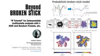
t-SNE Low-Dimensional Visualization of features
Data-driven identification of prognostic tumor subpopulations using spatially mapped t-
SNE of mass spectrometry imaging data https://doi.org/10.1073/pnas.1510227113

t-SNE R Implementation
t-SNE (Cited by 5394, in Python, in R)
Now that you have an understanding of what is
dimensionality reduction, let’s look at how we can
use t-SNE algorithm for reducing dimensions.
Following are a few dimensionality reduction
algorithms that you can check out:
●
PCA (linear)
●
t-SNE (non-parametric/ nonlinear)
●
Sammon mapping (nonlinear)
●
Isomap (nonlinear)
●
LLE (nonlinear)
●
CCA (nonlinear)
●
SNE (nonlinear)
●
MVU (nonlinear)
It’s quite simple actually, t-SNE a non-linear
dimensionality reduction algorithm finds patterns in
the data by identifying observed clusters based on
similarity of data points with multiple features. But it
is not a clustering algorithm it is a dimensionality
reduction algorithm.
This is because it maps the multi-dimensional data
to a lower dimensional space, the input features are
no longer identifiable. Thus you cannot make any
inference based only on the output of t-SNE. So
essentially it is mainly a data exploration and
visualization technique.
But t-SNE can be used in the process of
classification and clustering by using its output as
the input feature for other classification algorithms.

t-SNE Parameters
https://www.rdocumentation.org/packages/Rtsne/versions/0.13/topics/Rtsne

t-SNE fx the random seed for reproducibility
set.seed(42) # Sets seed for reproducibility
https://cran.r-project.org/web/packages/Rtsne/README.h
tml
https://doi.org/10.1016/j.celrep.2015.12.082: used a fixed random seed to"
make sure the t-SNE plot would be reproducible (parameter random_state =
254 in the scikit-learn implementation of t-SNE)."

t-SNE How to use
Check out the
excellent demo
https://distill.pub/2016/mis
read-tsne/

t-SNE Parameters in Demo https://distill.pub/2016/misread-tsne/
Perplexity
Tuneable parameter, “perplexity,” which says (loosely) how
to balance attention between local and global aspects of
your data. The parameter is, in a sense, a guess about the
number of close neighbors each point has. A low perplexity
means we care about local scale and focus on the closest
other points. High perplexity takes more of a “big picture”
approach.
But the story is more nuanced than that.
Getting the most from t-SNE may mean
analyzing multiple plots with different
perplexities.

t-SNE Parameters in Demo https://distill.pub/2016/misread-tsne/
No of Iterations
If you see a t-SNE plot with strange “pinched” shapes, chances are
the process was stopped too early.

t-SNE How about preprocessing/transformation
Bits from:
https://www.reddit.com/r/MachineLearning/comments/5ygh
1q/d_data_preprocessing_tips_for_tsne/
JamesLi2017
t-SNE is sensitive to feature-wise normalization; and no
theory says that such normalization will in general improve or
degrade results, it fully depends on your data and
expectation. If you can make more sense with maps from
un-normalized data, then it indicates that normalization is not
good for your study.
1 year ago
Would you mind elaborating just a bit as to what exactly you
mean by ranking pairwise distances?
Compute the pairwise Euclidean distances before
normalization, rank the values (lets call these indices x).
Then compute the pairwise Euclidean distances after
normalization, and rank them by x, lets call these values y. If
you plot(x,y) you will see that the resulting function is not
monotonic, i.e. rank order was not preserved.
Features might have quite
different ranges
Dimensionality reduction (PCA, tSNE)
- Let s encode the categorical variables and try again.'
Encoding categorical variables: one-hot and beyond

Preprocessing in R
https://www.displayr.com/using-t-sne-to
-visualize-data-before-prediction/
Because the distributions
are distance based, all
the data must be
numeric. You should
convert categorical
variables to numeric ones
by binary encoding or a
similar method. It is also
often useful to normalize
the data, so each variable
is on the same scale.
This avoids variables with
a larger numeric range
dominating the analysis.
Featurewise Z-score normalization for example
https://www.r-bloggers.com/r-tutorial-series-centering-variable
s-and-generating-z-scores-with-the-scale-function/
R Tutorial Series: Centering Variables
and Generating Z-Scores with the
Scale() Function
https://stackoverflow.com/questions/15215457/standardize-data-columns-in-r
COLUMN NORMALIZATION
library(caret)
# Assuming goal class is column 10
preObj <- preProcess(data[, -10], method=c("center", "scale"))
newData <- predict(preObj, data[, -10])
What is the purpose of row normalization
The main point is that normalizing rows can be detrimental to
any subsequent analysis, such as nearest-neighbor or k-
means. For simplicity, I will keep the answer specific to
mean-centering the rows.

t-SNE use as input for a classifer
t-SNE (Cited by 5394, in Python, in R)
Experimental results showed that the proposed new
algorithm applied to facial recognition gained the better
performance compared with those traditional algorithms,
such as PCA, LDA, LLE and SNE. [Yi et al. 2013]
The flowchart for implementing such a combination on the
data could be as follows:
Preprocessing → need to transform ordinal to numerical?
normalization → whiten for t-SNE?
→t-SNE classification algorithm→
PCA LDA LLE SNE t-SNE
SVM 73.5% 74.3% 84.7% 89.6% 90.3%
AdaboostM2 75.4% 75.9% 87.7% 90.6% 94.5%
adam2: Implementation of AdaBoost.M2In
ebmc: Ensemble-Based Methods for Class Imbalance Problem
ASurveyofseveraloftheAdaboostvariantscanbefoundinthepaper,
'SurveyonBoostingAlgorithmsforSupervisedandSemi-supervisedLearning,'Artur Ferreira.
pat:“Theother variantsarecoveredinthepaper,butlessfrequentlymentionedincommon
literature.AsIunderstandit,GentleAdaboostproducesamorestableensemblemodel.The
AdaBoost.M1andAdaBoost.M2modelsareextensionstomulti-classclassifcations(withM2
overcomingarestrictiononthemaximumerrorweightsofclassifersfromM1). “
"ExperimentswithaNewBoosting Algorithm,"YoavFreundandRobertE.Schapire.

t-SNE tweaks for classifcation
Set to 3
Might be better for classification?
Worse for visualization
DATA ANALYSIS RESOURCES
MACHINE LEARNING
The
Comprehensive
Guide for Feature
Engineering
POSTED AUGUST 28, 2016 PIUSH VAISH
More advanced Feature selection algorithms
may search subsets of features by trial and
error, creating and evaluating models
automatically in pursuit of the objectively
most predictive sub-group of features.
Regularization methods like LASSO and
ridge regression may also be considered
algorithms with feature selection baked in,
as they actively seek to remove or discount
the contribution of features as part of the
model building process.

Feature Selection for classifcation
Maybe your visual field
measurements are just
very noisy and do not
correlate with anything?
Feature Selection with the Caret R Packag
e
EFS: an ensemble feature selection tool im
plemented as R-packag
Easy feature selection for beginners in R
Venn diagram for the results obtained by different Feature Selection methods (from
the R library VennDiagram
https://doi.org/10.1038/srep19256

Classifers you can try some other multiclass classifers
RPubs - Intro to Machine
Learning for Classification
: Random Forests
Random Forest (RF) classification was performed
in the R environment using the randomForest
package.
https://doi.org/10.1038/srep31479
A Simple XGBoost Tutorial Using the Iris Dataset
KDnuggets

t-SNE/Random Forests
Single-Cell RNA-Sequencing Reveals a Continuous
Spectrum of Differentiation in Hematopoietic Cells
IainC.Macaulayetal. (2016)
function.

xyz Forests for other tasks as well

Outlier Forests identify outlier patients
An anomaly detection approach for the
identification of DME patients using spectral
domain optical coherence tomography images
DésiréSidibéetal.(2017)
ComputerMethodsandProgramsinBiomedicineVolume 139, February2017, Pages109-117
https://doi.org/10.1016/j.cmpb.2016.11.001
Isolation based anomaly detection using‐
nearest neighbor ensembles‐
Tharindu R. Bandaragoda, KaiMing, TingDavid, AlbrechtFei,TonyLiu, Ye Zhu, Jonathan R. Wells
ComputationalIntelligence(2018)
https://doi.org/10.1111/coin.12156 ← Isolationforest
Outlier detection for patient monitoring and
alerting
MilosHauskrecht, Iyad Batal, Michal Valko, ShyamVisweswaran, Gregory F. Cooper,GillesClermonte
Journal ofBiomedical InformaticsVolume 46, Issue 1, February 2013, Pages47-55
The investigation of
new, more suitable
feature sets that
characterize complex
time-series data may
lead to further
improvements and
better coverage of
patient management
actions with such
models.

Outlier Forests identify outlier patients 2#
A parameter based growing ensemble of self-
organizing maps for outlier detection in healthcare
Samir Elmougy, M. Shamim Hossain, Ahmed S. Tolba, Mohammed F. Alhamid, Ghulam Muhammad
Cluster Computing (2017)
https://doi.org/10.1007/s10586-017-1327-0

Clustering when your diagnosis code is ambiguous itself

Clustering electronic phenotyping 1#
Semi-supervised learning of the electronic
health record for phenotype stratification
BrettK.Beaulieu-Jones,CaseyS.Greene,thePooledResourceOpen-Access
ALSClinicalTrialsConsortium
Journal ofBiomedical InformaticsVolume 64, December 2016, Pages168-178
Patient interactions with health care providers result in entries to electronic
health records (EHRs). EHRs were built for clinical and billing purposes but
contain many data points about an individual. Mining these records provides
opportunities to extract electronic phenotypes, which can be paired with
genetic data to identify genes underlying common human diseases. This task
remains challenging: high quality phenotyping is costly and requires physician
review; many felds in the records are sparsely flled; and our defnitions
ofdiseasesarecontinuingtoimproveovertime.
Future work will focus on developing tools to examine and interpret
constructed phenotypes (hidden nodes) and clusters. In addition, we will
develop a framework for evaluating the signifcance of constructed
clusters for genotype to phenotype association. We anticipate high weights
indicate important contributors to node construction revealing relevant
combinations of input features. Finally we will construct a scheme for
determiningoptimalhyper parameter (i.e.hiddennodecount)selection
Case vs. Control clustering via principal components analysis
and t-distributed stochastic neighbor embedding

Clustering electronic phenotyping 2#
Flexible, cluster-based analysis of
the electronic medical record of
sepsis with composite mixture
models
MichaelB.Mayhew,BrendenK.Petersen,AnaPaulaSales,John
D.Greene,VincentX.Liu,ToddS.Wasson
Journal ofBiomedical InformaticsVolume 78, February2018, Pages33-42
In the case of sepsis, a debilitating, dysregulated host response
to infection, extracting subtle, uncataloged clinical phenotypes
from the EMR with statistical machine learning methods has the
potential to impact patient diagnosis and treatment early in the
courseoftheir hospitalization.
Here, we describe an unsupervised, probabilistic
framework called a composite mixture model that can
simultaneously accommodate the wide variety of observations
frequently observed in EMR datasets, characterize
heterogeneous clinical populations, and handle missing
observations. We demonstrate the efcacy of our approach on a
large-scale sepsis cohort, developing novel techniques built on
our model-based clusters to track patient mortality risk over
time and identify physiological trends and distinct subgroups
of the dataset associated with elevated risk of mortality during
hospitalization.
Estimated differences between cluster-specific
and population values of each feature. The
dots represent the estimated difference while
whiskers represent the 95% confidence interval
as computed by Wilcoxon rank-sum tests. The
lack of an overlap between these intervals and
a difference of 0 (gray line) reflects a
significant difference in cluster-specific values
of the feature as compared to the overall
population.

Go “FULL-ON Deep Learning” Structure+Function

Visual Fields Deep learnifed already 1#
2846 — B0449 A deep-learning
based automatic glaucoma
identification
SerifeSedaS.Kucur,M.Abegg,S.Wolf,R.Sznitman
1 ARTORG Center, University ofBern, Bern, Switzerland;
2 DepartmentofOpthalmology, Inselspital Bern, Bern, Switzerland
ARVO 2017 poster for deep learning in visual field
assessment
Şerife Seda Kucur Ergünay
Designingmachinelearningalgorithmstoimprovethe
acquisitionanddiagnosistoolsfor Glaucomamanagement.
FollowingareincludedwithinthePhDstudy:
-Designingnewperimetrystrategiesforaccuratevisualfeld
acquisitionleveragingtoolsfromreinforcementlearning,
sparseapproximation,graphicalmodels,auto-encoders
-EarlyGlaucomadetectionfromvisualfeldsusingdeep
learningapproach
-Predictingvisualfelds/Glaucomaprogression
frompatienthistoryviaLSTMs
Topic: lstm-neural-networks · GitHub
umbertogriffo / Predictive-Maintenance-using-LSTM
Example of Multiple Multivariate Time Series Prediction with LSTM
Recurrent Neural Networks in Python with Keras.
kinect59/Spatio-Temporal-LSTM - GitHub
Spatio-Temporal LSTM with Trust Gates for 3D Human Action
Recognition. – J Liu - 2016 - Cited by 179
blackeagle01 / Abnormal_Event_Detection
Abnormal Event Detection in Videos using SpatioTemporal AutoEncoder
Structural-RNN: Deep Learning on Spatio-Temporal Graphs
– Cited by 126
Videos as Space-Time Region Graphs
X Wang, A Gupta - arXiv preprint arXiv:1806.01810, 2018 How do humans
recognize the action opening a book ? We argue that there are two" "
important cues: modeling temporal shape dynamics and modeling
functional relationships between humans and objects. In this paper, we
propose to represent videos as space-time

Visual Fields Deep learnifed already 2#
Forecasting Future Humphrey Visual
Fields Using Deep Learning
JoanneC.Wen,CeciliaS.Lee,PearseA.Keane,SaXiao,YueWu,
ArielRokem,PhilipP.Chen,AaronY.Lee
(Submitted on 2 Apr 2018)
All datapoints from consecutive 24-2 HVFs from
1998 to 2018 were extracted from a University of
Washington database. More than 1.7 million
perimetry points were extracted to the hundredth
decibelfrom32,44324-2HVFs.
Clinical dataset combination selection was done
by taking the best performing model in the previous
step and testing every possible combinationof clinical
predictor variables. Categorical variables such as
eye and gender were appended in a one-hot vector
format to the input tensor and continuous
variables were encoded as a single additional
tensor face with every cell encodedasthecontinuous
value

Clinical Variables Combine with Images 1#
Glaucomadiagnosisbasedonbothhidden
featuresanddomainknowledgethroughdeep
Non-image features
from case report
Features such as age,
intraocular pressure,
eyesight and
symptoms are also
extracted. We regard
them as non-image
features for
simplicity. For age,
intraocular pressure
and eyesight features,
we just use the raw
numerical values from
case reports.

Clinical Variables Combine with Images 2#
An Ophthalmology Clinical Decision Support
System Based on Clinical Annotations,
Ontologies and Images (23 July 2018) José N.
Galveia ; Antonio Travassos ; Luis A. da Silva
Cruz.
https://doi.org/10.1109/CBMS.2018.00024
We explore a multimodal electronic health record dataset (n = 2348 cases and n = 2348
controls) and propose a new classifer model based on Random Forrest Classifers for
recommendation of an ophthalmic procedure (intravitreal injection of bevacizumab). The
dataset comprises structured demographic data, unstructured textual annotations, and
clinical images (optical coherence tomography, slit lamp photography and scanning laser
ophthalmoscopy).

Spatiotemporal inspiration Beyond Retina

Deep Forecast Spatiotemporal Forecasting
Deep Forecast:
Deep Learning-based Spatio-
Temporal Forecasting
Amir Ghaderi,BorhanM.Sanandaji,
FaezehGhaderi
(Submitted on 2 Apr 2018)
https://arxiv.org/pdf/1707.08110.pdf
https://github.com/amirstar/Deep-Forecast
Deep-Forecast/multiLSTM.py

Deep Forecast Spatiotemporal Forecasting
Deep Learning for Spatio-Temporal
Modeling: Dynamic Traffic Flows
and High Frequency Trading
MatthewF.Dixon,NicholasG.Polson,VadimO.Sokolov
(revised7May2018)

Beyond Broken Stick Modeling: R Tutorial for interpretable multivariate analysis

Empfohlen

Empfohlen

Weitere ähnliche Inhalte

Was ist angesagt?

Was ist angesagt? (15)

Ähnlich wie Beyond Broken Stick Modeling: R Tutorial for interpretable multivariate analysis

Ähnlich wie Beyond Broken Stick Modeling: R Tutorial for interpretable multivariate analysis (20)

Mehr von PetteriTeikariPhD

Mehr von PetteriTeikariPhD (16)

Kürzlich hochgeladen

Kürzlich hochgeladen (20)

Beyond Broken Stick Modeling: R Tutorial for interpretable multivariate analysis