Dynamic New Keynesian

1. Credit Spreads and Monetary Policy∗
Vasco C´rdia†
u Michael Woodford‡
Federal Reserve Bank of New York Columbia University
May 28, 2009
Abstract
We consider the desirability of modifying a standard Taylor rule for a cen-
tral bank’s interest-rate policy to incorporate either an adjustment for changes
in interest-rate spreads (as proposed by Taylor, 2008, and by McCulley and
Toloui, 2008) or a response to variations in the aggregate volume of credit (as
proposed by Christiano et al., 2007). We consider the consequences of such
adjustments for the way in which policy would respond to a variety of types
of possible economic disturbances, including (but not limited to) disturbances
originating in the financial sector that increase equilibrium spreads and con-
tract the supply of credit. We conduct our analysis using the simple DSGE
model with credit frictions developed in C´rdia and Woodford (2009), and com-
u
pare the equilibrium responses to a variety of disturbances under the modified
Taylor rules to those under a policy that would maximize average expected
utility. According to our model, either type of adjustment, if of an appropriate
magnitude, can improve equilibrium responses to disturbances originating in
the financial sector. However, neither simple rule of thumb is ideal even in
this case, and the specific adjustments that would best improve the response
to purely financial disturbances are less desirable in the case of other types of
disturbances.
∗
Prepared for the FRB-JMCB research conference “Financial Markets and Monetary Policy,”
Washington, DC, June 4-5, 2009. We thank Argia Sbordone and John Taylor for helpful discussions,
and the NSF for research support of the second author. The views expressed in this paper are those
of the authors and do not necessarily reflect positions of the Federal Reserve Bank of New York or
the Federal Reserve System.
†
E-mail : vasco.curdia@ny.frb.org
‡
E-mail : michael.woodford@columbia.edu

2. The recent turmoil in financial markets has confronted the central banks of the
world with a number of unusual challenges. To what extent do standard approaches
to the conduct of monetary policy continue to provide reasonable guidelines under
such circumstances? For example, the Federal Reserve aggressively reduced its oper-
ating target for the federal funds rate in late 2007 and January 2008, though official
statistics did not yet indicate that real GDP was declining, and according to many
indicators inflation was if anything increasing; a simple “Taylor rule” (Taylor, 1993)
for monetary policy would thus not seem to have provided any ground for the Fed’s
actions at the time. Obviously, they were paying attention to other indicators than
these ones alone, some of which showed that serious problems had developed in the
financial sector.1 But does a response to such additional variables make sense as a
general policy? Should it be expected to lead to better responses of the aggregate
economy to disturbances more generally?
Among the most obvious indicators of stress in the financial sector since August
2007 have been the unusual increases in (and volatility of) the spreads between the
interest rates at which different classes of borrowers are able to fund their activities.2
Indeed, McCulley and Toloui (2008) and Taylor (2008) have proposed that the in-
tercept term in a “Taylor rule” for monetary policy should be adjusted downward
in proportion to observed increases in spreads. Similarly, Meyer and Sack (2008)
propose, as a possible account of recent U.S. Federal Reserve policy, a Taylor rule
in which the intercept — representing the Fed’s view of “the equilibrium real funds
rate” — has been adjusted downward in response to credit market turmoil, and use
the size of increases in spreads in early 2008 as a basis for a proposed magnitude of
the appropriate adjustment. A central objective of this paper is to assess the degree
to which a modification of the classic Taylor rule of this kind would generally improve
the way in which the economy responds to disturbances of various sorts, including
in particular to those originating in the financial sector. Our model also sheds light
on the question whether it is correct to say that the “natural” or “neutral” rate
of interest is lower when credit spreads increase (assuming unchanged fundamentals
otherwise), and to the extent that it is, how the size of the change in the natural rate
compares to the size of the change in credit spreads.
Other authors have argued that if financial disturbances are an important source
1
For a discussion of the FOMC’s decisions at that time by a member of the committee, see
Mishkin (2008).
2
See, for example, Taylor and Williams (2008a, 2008b).
1

3. of macroeconomic instability, a sound approach to monetary policy will have to pay
attention to the balance sheets of financial intermediaries. It is sometimes suggested,
for example, that a Taylor rule that is modified to include a response to variations in
some measure of aggregate credit would be an improvement upon conventional policy
advice (see, e.g., Christiano et al., 2007). We also consider the cyclical variations
in aggregate credit that should be associated with both non-financial and financial
disturbances, and the desirability of a modified Taylor rule that responds to credit
variations in both of these cases.
Many of the models used both in theoretical analyses of optimal monetary policy
and in numerical simulations of alternative policy rules are unsuitable for the analysis
of these issues, because they abstract altogether from the economic role of financial
intermediation. Thus it is common to analyze monetary policy in models with a
single interest rate (of each maturity) — “the” interest rate — in which case we
cannot analyze the consequences of responding to variations in spreads, and with a
representative agent, so that there is no credit extended in equilibrium and hence
no possibility of cyclical variations in credit. In order to address the questions that
concern us here, we must have a model of the monetary transmission mechanism
with both heterogeneity (so that there are both borrowers and savers at each point
in time) and segmentation of the participation in different financial markets (so that
there can exist non-zero credit spreads).
The model that we use is one developed in C´rdia and Woodford (2009), as a rel-
u
atively simple generalization of the basic New Keynesian model used for the analysis
of optimal monetary policy in sources such as Goodfriend and King (1997), Clarida
et al. (1999), and Woodford (2003). The model is still highly stylized in many re-
spects; for example, we abstract from the distinction between the household and firm
sectors of the economy, and instead treat all private expenditure as the expenditure
of infinite-lived household-firms, and we similarly abstract from the consequences of
investment spending for the evolution of the economy’s productive capacity, instead
treating all private expenditure as if it were all non-durable consumer expenditure
(yielding immediate utility, at a diminishing marginal rate). The advantage of this
very simple framework, in our view, is that it brings the implications of the credit
frictions into very clear focus, by using a model that reduces, in the absence of those
frictions, to a model that is both simple and already very well understood.
In section 1, we review the structure of the model, stressing the respects in which
2

4. the introduction of heterogeneity and imperfect financial intermediation requires the
equations of the basic New Keynesian model to be generalized, and discuss its nu-
merical calibration. We then consider the economy’s equilibrium responses to both
non-financial and financial disturbances under the standard Taylor rule, according to
this model. Section 2 then analyzes the consequences of modifying the Taylor rule,
to incorporate an automatic response to either changes in credit spreads or in a mea-
sure of aggregate credit. We consider the welfare consequences of alternative policy
rules, from the standpoint of the average level of expected utility of the heterogenous
households in our model. Section 3 then summarizes our conclusions.
1 A New Keynesian Model with Financial
Frictions
Here we briefly describe the model developed in C´rdia and Woodford (2009). (The
u
reader is referred to that paper for more details.) We stress the similarity between
the model developed there and the basic New Keynesian [NK] model, and show how
the standard model is recovered as a special case of the extended model. This sets
the stage for a quantitative investigation of the degree to which credit frictions of
an empirically realistic magnitude change the predictions of the model about the
responses to shocks other than changes in the severity of financial frictions.
1.1 Sketch of the Model
We depart from the assumption of a representative household in the standard model,
by supposing that households differ in their preferences. Each household i seeks to
maximize a discounted intertemporal objective of the form
∞ 1
E0 β t uτ t (i) (ct (i); ξ t ) − v τ t (i) (ht (j; i) ; ξ t ) dj ,
t=0 0
where τ t (i) ∈ {b, s} indicates the household’s “type” in period t. Here ub (c; ξ) and
us (c; ξ) are two different period utility functions, each of which may also be shifted by
the vector of aggregate taste shocks ξ t , and v b (h; ξ) and v s (h; ξ) are correspondingly
two different functions indicating the period disutility from working. As in the basic
NK model, there is assumed to be a continuum of differentiated goods, each produced
3

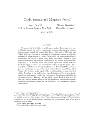
5. by a monopolistically competitive supplier; ct (i) is a Dixit-Stiglitz aggegator of the
household’s purchases of these differentiated goods. The household similarly supplies
a continuum of different types of specialized labor, indexed by j, that are hired by
firms in different sectors of the economy; the additively separable disutility of work
v τ (h; ξ) is the same for each type of labor, though it depends on the household’s type
and the common taste shock.
Each agent’s type τ t (i) evolves as an independent two-state Markov chain. Specif-
ically, we assume that each period, with probability 1 − δ (for some 0 ≤ δ < 1) an
event occurs which results in a new type for the household being drawn; otherwise it
remains the same as in the previous period. When a new type is drawn, it is b with
probability π b and s with probability π s , where 0 < π b , π s < 1, π b + π s = 1. (Hence
the population fractions of the two types are constant at all times, and equal to π τ
for each type τ .) We assume moreover that
ub (c; ξ) > us (c; ξ)
c c
for all levels of expenditure c in the range that occur in equilibrium. (See Figure
1, where these functions are graphed in the case of the calibration discussed below.)
Hence a change in a household’s type changes its relative impatience to consume,
given the aggregate state ξ t ; in addition, the current impatience to consume of all
households is changed by the aggregate disturbance ξ t . We also assume that the
marginal utility of additional expenditure diminishes at different rates for the two
types, as is also illustrated in the figure; type b households (who are borrowers in
equilibrium) have a marginal utility that varies less with the current level of expendi-
ture, resulting in a greater degree of intertemporal substitution of their expenditures
in response to interest-rate changes. Finally, the two types are also assumed to differ
in the marginal disutility of working a given number of hours; this difference is cali-
brated so that the two types choose to work the same number of hours in steady state,
despite their differing marginal utilities of income. For simplicity, the elasticities of
labor supply of the two types are not assumed to differ.
The coexistence of the two types with differing impatience to consume creates
a social function for financial intermediation. In the present model, as in the basic
New Keynesian model, all output is consumed either by households or by the gov-
ernment;3 hence intermediation serves an allocative function only to the extent that
3
The “consumption” variable is therefore to be interpreted as representing all of private expendi-
4

6. there are reasons for the intertemporal marginal rates of substitution of households
to differ in the absence of financial flows. The present model reduces to the standard
representative-household model in the case that one assumes that ub (c; ξ) = us (c; ξ)
and v b (h; ξ) = v s (h; ξ).
We assume that most of the time, households are able to spend an amount dif-
ferent from their current income only by depositing funds with or borrowing from
financial intermediaries, and that the same nominal interest rate id is available to all
t
savers, and that a (possibly) different nominal interest it is available to all borrowers,4
b
independent of the quantities that a given household chooses to save or to borrow.
(For simplicity, we also assume that only one-period riskless nominal contracts with
the intermediary are possible for either savers or borrowers.) The assumption that
households cannot engage in financial contracting other than through the intermedi-
ary sector represents the key financial friction.
The analysis is simplified by allowing for an additional form of financial contract-
ing. We assume that households are able to sign state-contingent contracts with one
another, through which they may insure one another against both aggregate risk and
the idiosyncratic risk associated with a household’s random draw of its type, but
that households are only intermittently able to receive transfers from the insurance
agency; between the infrequent occasions when a household has access to the insur-
ance agency,5 it can only save or borrow through the financial intermediary sector
mentioned in the previous paragraph. The assumption that households are eventu-
ally able to make transfers to one another in accordance with an insurance contract
signed earlier means that they continue to have identical expectations regarding their
marginal utilities of income far enough in the future, regardless of their differing type
ture, not only consumer expenditure. In reality, one of the most important reasons for some economic
units to wish to borrow from others is that the former currently have access to profitable investment
opportunities. Here we treat these opportunities as if they were opportunities to consume, in the
sense that we suppose that the expenditure opportunities are valuable to the household, but we
abstract from any consequences of current expenditure for future productivity. For discussion of
the interpretation of “consumption” in the basic New Keynesian model, see Woodford (2003, pp.
242-243).
4
Here “savers” and “borrowers” identify households according to whether they choose to save or
borrow, and not by their “type”.
5
For simplicity, these are assumed to coincide with the infrequent occasions when the household
draws a new “type”; but the insurance payment is claimed before the new type is known, and cannot
be contingent upon the new type.
5

7. histories.
As long as certain inequalities discussed in our previous paper are satisfied,6 it
turns out that in equilibrium, type b households choose always to borrow from the
intermediaries, while type s households deposit their savings with them (and no
one chooses to do both, given that ib ≥ id at all times). Moreover, because of the
t t
asymptotic risk-sharing, one can show that all households of a given type at any
point in time have a common marginal utility of real income (which we denote λτ for
t
τ
households of type τ ) and choose a common level of real expenditure ct . Household
optimization of the timing of expenditure requires that the marginal-utility processes
{λτ } satisfy the two Euler equations
t
1 + ib
λb = βEt
t
t
[δ + (1 − δ) π b ] λb + (1 − δ) π s λs
t+1 t+1 , (1.1)
Πt+1
1 + id
λs = βEt
t
t
(1 − δ) π b λb + [δ + (1 − δ) π s ] λs
t+1 t+1 (1.2)
Πt+1
in each period. Here Πt ≡ Pt /Pt−1 is the gross inflation rate, where Pt is the Dixit-
Stiglitz price index for the differentiated goods produced in period t. Note that each
equation takes into account the probability of switching type from one period to the
next.
Assuming an interior choice for consumption by households of each type, the
expenditures of the two types must satisfy
λb = ub (cb ),
t t λs = us (cs ),
t t
which relations can be inverted to yield demand functions
cb = cb (λb ; ξ t ),
t t cs = cs (λs ; ξ t ).
t t
Aggregate demand Yt for the Dixit-Stiglitz composite good is then given by
Yt = π b cb (λb ; ξ t ) + π s cs (λs ; ξ t ) + Gt + Ξt ,
t t (1.3)
where Gt indicates the (exogenous) level of government purchases and Ξt indicates
resources consumed by the intermediary sector (discussed further below). Equations
6
We verify that in the case of the numerical parameterization of the model discussed below, these
inequalities are satisfied at all times, in the case of small enough random disturbances of any of the
kinds discussed.
6

8. (1.1)–(1.2) together with (1.3) indicate the way in which the two real interest rates
of the model affect aggregate demand. This system directly generalizes the relation
that exists in the basic NK model as a consequence of the Euler equation of the
representative household.
It follows from the same assumptions that optimal labor supply in any given
period will be the same for all households of a given type. Specifically, any household
of type τ will supply hours hτ (j) of labor of type j, so as to satisfy the first-order
condition
µw vh (hτ (j); ξ t ) = λτ Wt (j)/Pt ,
t
τ
t t (1.4)
where Wt (j) is the wage for labor of type j, and the exogenous factor µw represents a
t
possible “wage markup” (the sources of which are not further modeled). Aggregation
of the labor supply behavior of the two types is facilitated if, as in Benigno and
Woodford (2005), we assume the isoelastic functional form
ψ τ 1+ν ¯ −ν
v τ (h; ξ t ) ≡ h Ht , (1.5)
1+ν
¯
where {Ht } is an exogenous labor-supply disturbance process (assumed common to
the two types, for simplicity); ψ b , ψ s > 0 are (possibly) different multiplicative coef-
ficients for the two types; and the coefficient ν ≥ 0 (inverse of the Frisch elasticity
of labor supply) is assumed to be the same for both types. Solving (1.4) for the
competitive labor supply of each type and aggregating, we obtain
1/ν
˜
λt Wt (j)
¯
ht (j) = Ht
ψµw Pt
t
for the aggregate supply of labor of type j, where
ν
˜ λb λs
λt ≡ ψ π b ( t )1/ν + π s ( t )1/ν , (1.6)
ψb ψs
−ν
−1/ν
ψ ≡ πbψb + π s ψ −1/ν
s .
We furthermore assume an isoelastic production function
yt (i) = Zt ht (i)1/φ
for each differentiated good i, where φ ≥ 1 and Zt is an exogenous, possibly time-
varying productivity factor, common to all goods. We can then determine the demand
7

9. for each differentiated good as a function of its relative price using the usual Dixit-
Stiglitz demand theory, and determine the wage for each type of labor by equating
supply and demand for that type. We finally obtain a total wage bill
1+ω y
Pt Yt
Wt (j)ht (j)dj = ψµw
t ∆t , (1.7)
˜ ¯
λt Htν Zt
where ω y ≡ φ(1 + ν) − 1 ≥ 0 and
−θ(1+ω y )
pt (i)
∆t ≡ di ≥ 1
Pt
is a measure of the dispersion of goods prices (taking its minimum possible value, 1,
if and only if all prices are identical), in which θ > 1 is the elasticity of substitution
among differentiated goods in the Dixit-Stiglitz aggregator. Note that in the Calvo
model of price adjustment, this dispersion measure evolves according to a law of
motion
∆t = h(∆t−1 , Πt ), (1.8)
where the function h(∆, Π) is defined as in Benigno and Woodford. Finally, since
households of type τ supply fraction
1
λτ ψ
t
ν
πτ
˜t ψτ
λ
of total labor of each type j, they also receive this fraction of the total wage bill each
period. This observation together with (1.7) allows us to determine the wage income
of each household at each point in time.
These solutions for expenditure on the one hand and wage income on the other
for each type allow us to solve for the evolution of the net saving or borrowing of
households of each type. We let the credit spread ω t ≥ 0 be defined as the factor
such that
1 + ib = (1 + id )(1 + ω t ),
t t (1.9)
and observe that in equilibrium, aggregate deposits with intermediaries must equal
aggregate saving by type s households in excess of bg , the real value of (one-period,
t
riskless nominal) government debt (the evolution of which is also specified as an
8

10. exogenous disturbance process7 ), which in equilibrium must pay the same rate of
interest id as deposits with intermediaries. It is then possible to derive a law of
t
motion for aggregate private borrowing bt , of the form
(1 + π b ω t )bt = π b π s B(λb , λs , Yt , ∆t ; ξ t ) − π b bg
t t t
1 + id
+δ[bt−1 (1 + ω t−1 ) + π b bg ] t−1
t
, (1.10)
Πt
where the function B (defined in C´rdia and Woodford, 2009) indicates the amount
u
by which the expenditure of type b households in excess of their current wage income
is greater than the expenditure of type s households in excess of their current wage
income. This equation, which has no analog in the representative-household model,
allows us to solve for the dynamics of private credit in response to various types
of disturbances. It becomes important for the general-equilibrium determination of
other variables if (as assumed below) the credit spread and/or the resources used by
intermediaries depend on the volume of private credit.
We can similarly use the above model of wage determination to solve for the
marginal cost of producing each good as a function of the quantity demanded of it,
again obtaining a direct generalization of the formula that applies in the representative-
household case. This allows us to derive equations describing optimal price-setting by
the monopolistically competitive suppliers of the differentiated goods. As in the basic
NK model, Calvo-style staggered price adjustment then implies an inflation equation
of the form
Πt = Π(zt ), (1.11)
where zt is a vector of two forward-looking variables, recursively defined by a pair of
relations of the form
zt = G(Yt , λb , λs ; ξ t ) + Et [g(Πt+1 , zt+1 )],
t t (1.12)
where the vector-valued functions G and g are defined in C´rdia and Woodford (2009).
u
(Among the arguments of G, the vector of exogenous disturbances ξ t now includes
an exogenous sales tax rate τ t , in addition to the disturbances already mentioned.)
7
Our model includes three distinct fiscal disturbances, the processes Gt , τ t , and bg , each of which
t
can be independently specified. The residual income flow each period required to balance the
government’s budget is assumed to represent a lump-sum tax or transfer, equally distributed across
households regardless of type.
9

11. These relations are of exactly the same form as in the basic NK model, except
that two distinct marginal utilities of income are here arguments of G; in the case
that λb = λs = λt , the relations (1.12) reduce to exactly the ones in Benigno and
t t
Woodford (2005). The system (1.11)–(1.12) indicates the nature of the short-run
aggregate-supply trade-off between inflation and real activity at a point in time,
given expectations regarding the future evolution of inflation and of the variables
{zt }.
It remains to specify the frictions associated with financial intermediation, that
determine the credit spread ω t and the resources Ξt consumed by the intermediary
sector. We allow for two sources of credit spreads — one of which follows from an
assumption that intermediation requires real resources, and the other of which does
not — which provide two distinct sources of “purely financial” disturbances in our
model. On the one hand, we assume that real resources Ξt (bt ) are consumed in
the process of originating loans of real quantity bt , and that these resources must be
produced and consumed in the period in which the loans are originated. The function
Ξt (bt ) is assumed to be non-decreasing and at least weakly convex. In addition, we
suppose that in order to originate a quantity of loans bt that will be repaid (with
interest) in the following period, it is necessary for an intermediary to also make
a quantity χt (bt ) of loans that will be defaulted upon, where χt (bt ) is also a non-
decreasing, weakly convex function. (We assume that intermediaries are unable to
distinguish the borrowers who will default from those who will repay, and so offer
loans to both on the same terms, but that they are able to accurately predict the
fraction of loans that will not be repaid as a function of a given scale of expansion of
their lending activity.) Hence total (real) outlays in the amount bt + χt (bt ) + Ξt (bt )
are required8 in a given period in order to originate a quantity bt of loans that will
be repaid (yielding (1 + ib )bt in the following period). Competitive loan supply by
t
intermediaries then implies that
ω t = ω t (bt ) ≡ χt (bt ) + Ξt (bt ). (1.13)
It follows that in each period, the credit spread ω t will be a non-negative-valued,
8
It might be thought more natural to make the resource requirement Ξt a function of the total
quantity bt + χt (bt ) of loans that are originated, rather than a function of the “sound” loans bt .
But since under our assumptions bt + χt (bt ) is a (possibly time-varying) function of bt , it would in
any event be possible to express Ξt as a (possibly time-varying) function of bt , with the properties
assumed in the text.
10

12. non-decreasing function of the real volume of private credit bg . This function may shift
t
over time, as a consequence of exogenous shifts in either the resource cost function
Ξt or the default rate χt .9 Allowing these functions to be time-varying introduces the
possibility of “purely financial” disturbances, of a kind that will be associated with
increases in credit spreads and/or reduction in the supply of credit.
Finally, we assume that the central bank is able to control the deposit rate id (the
t
10
rate at which intermediaries are able to fund themselves), though this is no longer
also equal to the rate ib at which households are able to borrow, as in the basic NK
t
model. Monetary policy can then be represented by an equation such as
id = id (Πt , Yt ),
t t (1.14)
which represents a Taylor rule subject to exogenous random shifts that can be given
a variety of interpretations. (This is of course only one simple specification of mon-
etary policy; we consider central-bank reaction functions with additional arguments
in section 2.)
If we substitute the functions ω t (bt ) and Ξt (bt ) for the variables ω t and Ξt in the
above equations, then the system consisting of equations (1.1)–(1.3), (1.8)–(1.12),
and (1.14) comprise a system of 10 equations per period to determine the 10 endoge-
nous variables Πt , Yt , id , ib , λb , λs , bt , ∆t , and zt , given the evolution of the exogenous
t t t t
disturbances. The disturbances that affect these equations include the productivity
factor Zt ; the fiscal disturbances Gt , τ t , and bg ; a variety of potential preference shocks
t
(variations in impatience to consume, that may or may not equally affect households
of the two types, and variations in attitudes toward work, assumed to be common to
the two types) and variations in the wage markup µw ; purely financial shocks (shifts
t
in either of the functions Ξt (bt ) and χt (bt )); and monetary policy shocks (shifts in
the function it (Πt , Yt )). We consider the consequences of systematic monetary policy
9
Of course, these shifts must not be purely additive shifts, in order for the function ω t (bt ) to shift.
In our numerical work below, the two kinds of purely financial disturbances that are considered are
multiplicative shifts of the two functions.
10
If we extend the model by introducing central-bank liabilities that supply liquidity services to
the private sector, the demand for these liabilities will be a decreasing function of the spread between
id and the interest rate paid on central-bank liabilities (reserves). The central bank will then be
t
able to influence id by adjusting either the supply of its liabilities (through open-market purchases
t
of government debt, for example) or the interest rate paid on them. Here we abstract from this
additional complication by treating id as directly under the control of the central bank.
t
11

13. for the economy’s response to all of these types of disturbances below. Note that
this system of equations reduces to the basic NK model (as presented in Benigno and
Woodford, 2005) if we identify λb and λs and identify id and ib (so that the pair of
t t t t
Euler equations (1.1)–(1.2) reduces to a single equation, relating the representative
household’s marginal utility of income to the single interest rate); identify the two
expenditure functions cs (λ; ξ) and cb (λ; ξ); set the variables ω t and Ξt equal to zero
at all times; and delete equation (1.10), which describes the dynamics of a variable
(bt ) that has no significance in the representative-household case.
1.2 Log-Linearized Structural Equations
In our numerical analysis of the consequences of alternative monetary policy rules,
we plot impulse responses to a variety of shocks under a candidate policy rule. The
responses that we plot are linear approximations to the actual response, accurate in
the case of small enough disturbances. These linear approximations to the equilibrium
responses are obtained by solving a system of linear (or log-linear) approximations to
the model structural equations (including a linear equation for the monetary policy
rule). Here we describe some of these log-linearized structural equations, as they
provide further insight into the implications of our model, and facilitate comparison
with the basic NK model.
We log-linearize the model structural relations around a deterministic steady state
¯
with zero inflation each period, and a constant level of aggregate output Y . (We as-
sume that, in the absence of disturbances, the monetary policy rule (1.14) is consistent
with this steady state, though the small disturbances in the structural equations that
we consider using the log-linearized equations may include small departures from the
inflation target of zero.) These log-linear relations will then be appropriate for ana-
lyzing the consequences of alternative monetary policy rules only in the case of rules
consistent with an average inflation rate that is not too far from zero. But in C´rdia
u
and Woodford (2009), we show that under an optimal policy commitment (Ramsey
policy), the steady state is indeed the zero-inflation steady state. Hence all policy
rules that represent approximations to optimal policy will indeed have this property.
We express our log-linearized structural relations in terms of deviations of the
ˆ ¯
logarithms of quantities from their steady-state values (Yt ≡ log(Yt /Y ), etc.), the
inflation rate π t ≡ log Πt , and deviations of (continuously compounded) interest rates
12

14. from their steady-state values (ˆd ≡ log(1 + id /1 + ¯d ), etc.). We also introduce
ıt t ı
isoelastic functional forms for the utility of consumption of each of the two types,
which imply that
¯
cτ (λ; ξ t ) = Ctτ λ−στ
¯
for each of the two types τ ∈ {b, s}, where Ctτ is a type-specific exogenous distur-
bance (indicating variations in impatience to consume, or in the quality of spending
opportunities) and σ τ > 0 is a type-specific intertemporal elasticity of substitution.
Then as shown in C´rdia and Woodford (2009), log-linearization of the system
u
consisting of equations (1.1)–(1.3) allows us to derive an “intertemporal IS relation”
ˆ ˆ ˆ
Yt = −¯ (ˆavg − Et π t+1 ) + Et Yt+1 − Et ∆gt+1 − Et ∆Ξt+1
σ ıt
σ ˆ ˆ
−¯ sΩ Ωt + σ (sΩ + ψ Ω )Et Ωt+1 ,
¯ (1.15)
where
ˆavg ≡ π bˆb + π sˆd
ıt ıt ıt (1.16)
is the average of the interest rates that are relevant (at the margin) for all of the
savers and borrowers in the economy; gt is a composite “autonomous expenditure”
disturbance as in Woodford (2003, pp. 80, 249), taking account of the exogenous
¯ ¯
fluctuations in Gt , Ctb , and Cts (and again weighting the fluctuations in the spending
opportunities of the two types in proportion to their population fractions);
ˆ ˆb ˆs
Ωt ≡ λt − λt ,
the “marginal-utility gap” between the two types, is a measure of the inefficiency
of the intratemporal allocation of resources as a consequence of imperfect financial
intermediation; and
ˆ ¯ ¯
Ξt ≡ (Ξt − Ξ)/Y
measures departures of the quantity of resources consumed by the intermediary sector
from its steady-state level.11 In this equation, the coefficient
σ ≡ π b sb σ b + π s ss σ s > 0
¯ (1.17)
11 ˆ
We adopt this notation so that Ξt is defined even when the model is parameterized so that
¯ = 0.
Ξ
13

15. is a measure of the interest-sensitivity of aggregate demand, using the notation sτ for
the steady-state value of cτ /Yt ; the coefficient
t
sb σ b − ss σ s
sΩ ≡ π b π s
σ
¯
is a measure of the asymmetry in the interest-sensitivity of expenditure by the two
types; and the coefficient
ψ Ω ≡ π b (1 − χb ) − π s (1 − χs )
is also a measure of the difference in the situations of the two types. Here we use the
notation
χτ ≡ β(1 + rτ )[δ + (1 − δ)π τ ]
¯
for each of the two types, where rτ is the steady-state real rate of return that is
¯
relevant at the margin for type τ . Note that except for the presence of the last three
terms on the right-hand side (all of which are identically zero in a model without
financial frictions), equation (1.15) has the same form as the intertemporal IS relation
in the basic NK model; the only differences are that the interest rate that appears is
a weighted average of two interest rates (rather than simply “the” interest rate), the
elasticity σ is a weighted average of the corresponding elasticities for the two types of
¯
households (rather than the elasticity of expenditure by a representative household),
and the disturbance term gt involves a weighted average of the expenditure demand
¯
shocks Ctτ for the two types (rather than the corresponding shock for a representative
household).
Equation (1.15) is derived by taking a weighted average of the log-linearized forms
of the two Euler equations (1.1)–(1.2), and then using the log-linearized form of (1.3)
to relate average marginal utility to aggregate expenditure. If we instead subtract
the log-linearized version of (1.2) from the log-linearized (1.1), we obtain
Ωt = ω t + ˆ t Ωt+1 .
ˆ ˆ δE ˆ (1.18)
Here we define
ω t ≡ log(1 + ω t /1 + ω ),
ˆ ¯
so that the log-linearized version of (1.9) is
ˆb = ˆd + ω t .
ıt ıt ˆ (1.19)
14

16. and
ˆ ≡ χ + χ − 1 < 1.
δ b s
ˆ
Equation (1.18) can be “solved forward” for Ωt as a forward-looking moving aver-
age of the expected path of the credit spread ω t . This now gives us a complete theory
ˆ
of the way in which time-varying credit spreads affect aggregate demand, given an
expected forward path for the policy rate. One the one hand, higher current and/or
future credit spreads raise the expected path of ˆavg for any given path of the policy
ıt
ˆ
rate, owing to (1.19), and this reduces aggregate demand Yt according to (1.15). And
on the other hand, higher current and/or future credit spreads increase the marginal-
ˆ
utility gap Ωt , owing to (1.18), and (under the parameterization that we find most
realistic) this further reduces aggregate demand for any expected forward path for
ˆ
ˆavg , as a consequence of the Ωt terms in (1.15). The fact that larger credit spreads
ıt
reduce aggregate demand for a given path of the policy rate is consistent with the
implicit model behind the proposal of McCulley and Toloui (2008) and Taylor (2008).
But our model does not indicate, in general, that it is only the borrowing rate ib that
t
matters for aggregate demand determination. Hence there is no reason to expect that
the effect of an increased credit spread on aggregate demand can be fully neutral-
ized through an offsetting reduction of the policy rate, as the simple proposal of a
one-for-one offset seems to presume.
Log-linearization of the aggregate-supply block consisting of equations (1.11)–
(1.12) similarly yields a log-linear aggregate-supply relation of the form
ˆ ˆ ˆ σ ˆ
π t = κ(Yt − Ytn ) + βEt π t+1 + ut + ξ(sΩ + π b − γ b )Ωt − ξ¯ −1 Ξt , (1.20)
ˆ
where Ytn (the “natural rate of output”) is a composite exogenous disturbance term,
¯
a linear combination of the variations in gt , Ht and Zt (sources of variation in the
flexible-price equilibrium level of output that, in the absence of steady-state distor-
tions or financial frictions, correspond to variations in the efficient level of output),
while the additional exogenous disturbance term ut (the “cost-push shock”) is in-
stead a linear combination of the variations in µw and τ t (sources of variation in the
t
flexible-price equilibrium level of output that do not correspond to any change in the
15

17. efficient level of output).12 The coefficients in this equation are given by
b 1/ν
¯
ψλ
γ b ≡ πb ¯ > 0;
ψλ˜
b
1 − α 1 − αβ
ξ≡ > 0,
α 1 + ωy θ
where 0 < α < 1 is the fraction of prices that remain unchanged from one period to
the next; and
κ ≡ ξ(ω y + σ −1 ) > 0.
¯
Note that except for the presence of the final two terms on the right-hand side,
(1.20) is exactly the “New Keynesian Phillips curve” relation of the basic NK model
(as expounded, for example, in Clarida et al., 1999), and the definitions of both the
disturbance terms and the coefficient κ are exactly the same as in that model (except
that σ replaces the elasticity of the representative household). The two new terms,
¯
ˆ ˆ
proportional to Ωt and Ξt , respectively, are present only to the extent that there
are credit frictions. These terms indicate that, in addition to their consequences
for aggregate demand, variations in the size of credit frictions also have “cost-push”
effects on the short-run aggregate-supply tradeoff between aggregate real activity and
inflation.
Finally, the central-bank reaction function (1.14) can be log-linearized to yield
ıt ˆ
ˆd = φπ π t + φy Yt + m
t , (1.21)
where m is an exogenous disturbance term (to which we shall refer as a “monetary
t
policy shock”). Except for the disturbance, this is the form of linear rule recom-
mended by Taylor (1993). The implications of such a rule for the evolution of the
composite interest rate ˆavg that appears in the IS relation (1.15) can be derived by
ıt
using (1.19) to write
ˆavg = ˆd + π b ω t .
ıt ıt ˆ (1.22)
12
See C´rdia and Woodford (2009) for the precise definition of these composite disturbances. They
u
are in fact exactly the same as in the basic NK model (Woodford, 2003, chap. 3, or Benigno and
Woodford, 2005), except that σ defined in (1.17) replaces the corresponding intertemporal elasticity
¯
of expenditure of the representative household.
16

18. 1.3 Numerical Calibration
The numerical values for parameters that are used in our calculations below are
the same as in C´rdia and Woodford (2009). Many of the model’s parameters are
u
also parameters of the basic NK model, and in the case of these parameters we
assume similar numerical values as in the numerical analysis of the basic NK model
in Woodford (2003, Table 6.1.), which in turn are based on the empirical model of
Rotemberg and Woodford (1997). The new parameters that are also needed for the
present model are those relating to heterogeneity or to the specification of the credit
frictions. The parameters relating to heterogeneity are the fraction π b of households
that are borrowers, the degree of persistence δ of a household’s “type”, the steady-
state expenditure level of borrowers relative to savers, sb /ss , and the interest-elasticity
of expenditure of borrowers relative to that of savers, σ b /σ s .13
In the calculations reported here, we assume that π b = π s = 0.5, so that there
are an equal number of borrowers and savers. We assume that δ = 0.975, so that the
expected time until a household has access to the insurance agency (and its type is
drawn again) is 10 years. This means that the expected path of the spread between
lending and deposit rates for 10 years or so into the future affects current spending
decisions, but that expectations regarding the spread several decades in the future
are nearly irrelevant.
We calibrate the degree of heterogeneity in the steady-state expenditure shares
of the two types so that the implied steady-state debt ¯ is equal to 80 percent of
b
annual steady-state output.14 This value matches the median ratio of private (non-
financial, non-government, non-mortgage) debt to GDP over the period 1986-2008.15
This requires a ratio sb /ss = 1.27. We calibrate the value of σ b /σ s to equal 5. This
is an arbitrary choice, though the fact that borrowers are assumed to have a greater
willingness to substitute intertemporally is important, as this results in the prediction
that an exogenous tightening of monetary policy (a positive value of the residual m t
in (1.14)) results in a reduction in the equilibrium volume of credit bt (see Figures 2
13
Another new parameter that matters as a consequence of heterogeneity is the steady-state level
of government debt relative to GDP, ¯g /Y ; here we assume that ¯g = 0.
b ¯ b
14
In our quarterly model, this means that ¯ Y = 3.2.
b/ ¯
15
We exclude mortgage debt when calibrating the degree of heterogeneity of preferences in our
model, since mortgage debt is incurred in order to acquire an asset, rather than to consume current
produced goods in excess of current income.
17

19. and 5 below). This is consistent with VAR evidence on the effects of an identified
monetary policy shock on household borrowing.16
It is also necessary to specify the steady-state values of the functions ω(b) and
Ξ(b) that describe the financial frictions, in addition to making clear what kinds
of random perturbations of these functions we wish to consider when analyzing the
effects of “financial shocks.” We here present results for two cases. In each case, we
assume that the steady-state credit spread is due entirely to the marginal resource
cost of intermediation;17 but we do allow for exogenous shocks to the default rate,
and this is what we mean by the “financial shock” in Figures 10 through 12 below.18
In treating the “financial shock” as involving an increase in markups but no increase
in the real resources used in banking, we follow Gerali et al. (2008).19
The two cases considered differ in the specification of the (time-invariant) interme-
diation technology Ξ(b). In the case of a linear intermediation technology, we suppose
˜
that Ξ(b) = Ξb, while in the case of a convex intermediation technology, we assume
that
˜
Ξ(b) = Ξbη (1.23)
for some η > 1.20 In both cases, in our numerical analyses we assume a steady-state
16
See, for example, Den Haan et al. (2004).
17
We assume this in the results presented here because we do not wish to appear to have sought
to minimize the differences between a model with financial frictions and the basic NK model, and
the use of real resources by the financial sector (slightly) increases the differences between the two
models.
18
Note that our conclusions regarding both equilibrium and optimal responses to shocks other
than the “financial shock” are the same as in an economy in which the banking system is perfectly
competitive (and there are no risk premia), up to the linear approximation used in the numerical
results reported below.
19
These authors cite the Eurosystem’s quarterly Bank Lending Survey as showing that since
October 2007, banks in the euro area had “strongly increased the margins charged on average and
riskier loans” (p. 24).
20
One interpretation of this function is in terms of a monitoring technology of the kind assumed
in Goodfriend and McCallum (2007). Suppose that a bank produces monitoring according to a
−1 −1
Cobb-Douglas production function, k 1−η Ξη , where k is a fixed factor (“bank capital”), and
t
must produce a unit of monitoring for each unit of loans that it manages. Then the produced
goods Ξt required as inputs to the monitoring technology in order to manage a quantity b of loans
˜
will be given by a function of the form (1.23), where Ξ = k 1−η . A sudden impairment of bank
capital, treated as an exogenous disturbance, can then be represented as a random increase in the
˜
multiplicative factor Ξ. This is another form of “financial shock”, with similar, though not identical,
18

20. credit spread ω equal to 2.0 percentage points per annum,21 following Mehra et al.,
¯
22
(2008). (Combined with our assumption that “types” persist for 10 years on average,
¯ ¯b ¯s
this implies a steady-state “marginal utility gap” Ω ≡ λ /λ = 1.22, so that there
would be a non-trivial welfare gain from transferring further resources from savers
to borrowers.) In the case of the convex technology, we set η so that a one-percent
increase in the volume of credit increases the credit spread by one percentage point
(per annum).23 The assumption that η > 1 allows our model to match the prediction
of VAR estimates that an unexpected tightening of monetary policy is associated with
a slight reduction in credit spreads (see, e.g., Lown and Morgan, 2002, and Gerali et
al., 2008). We have chosen a rather extreme value for this elasticity in our calibration
of the convex-technology case, in order to make more visible the difference that a
convex technology makes for our results. (In the case of a smaller value of η, the
results for the convex technology are closer to those for the linear technology, and in
fact are in many respects similar to those for an economy with no financial frictions
at all.)
As a first exercise, we consider the implied equilibrium responses of the model’s
endogenous variables to the various kinds of exogenous disturbances, under the as-
sumption that monetary policy is described by a Taylor rule of the form (1.21). The
coefficients of the monetary policy rule are assigned the values φπ = 1.5 and φy = 0.524
as recommended by Taylor (1993).25 Among other disturbances, we consider the ef-
fects of random disturbances to the error term m in the monetary policy rule. In
t
section 2, we consider the predicted dynamics under a variety of other monetary
policy specifications as well.
In all of the cases that we consider, we assume that each of the exogenous distur-
effects as the default rate shock considered below.
21
In our quarterly numerical model, this means that we choose a value such that (1 + ω )4 = 1.02.
¯
22
Mehra et al. argue for this calibration by dividing the net interest income of financial intermedi-
aries (as reported in the National Income and Product Accounts) by a measure of aggregate private
credit (as reported in the Flow of Funds). As it happens, this value also corresponds to the median
spread between the FRB index of commercial and industrial loan rates and the federal funds rate,
over the period 1986-2007.
23
This requires that η = 51.6.
24
This is the value of φy if ˆd and π t are quoted as annualized rates, as in Taylor (1993). If,
ıt
ˆ
instead, (1.21) is written in terms of quarterly rates, then the coefficient on Yt is only 0.5/4.
25
See, for example, Taylor (2007) as an example of more recent advocacy of a rule with these same
coefficients.
19

21. bances ξ it evolves according to an AR(1) process,
ξ it = ρi ξ i,t−1 + it ,
where it is a mean-zero i.i.d. random process, and that these processes are indepen-
dent for the different disturbances i. We make various assumptions about the size of
the coefficient of serial correlation ρi and the standard deviation of the innovations
it , that are explained below.
1.4 Credit Frictions and the Propagation of Disturbances
We can explore the consequences of introducing financial frictions into our model by
considering the predicted responses to aggregate disturbances of a kind that also exist
in the basic NK model, and see how much difference to our results the allowance for
credit frictions makes. A special case in which we obtain a simple result is that in
which (i) Ξt is an exogenous process (i.e., independent of bt — there are no variable
resource costs of intermediation), and (ii) χt (b) is a linear function, χt (b) = χt b, at
˜
all times (i.e., the default rate is independent of the volume of lending), though the
default rate may vary (exogenously) over time. In this case, (1.13) implies that ω t
ˆ
will also be an exogenous process (equal to χt ), and (1.18) implies that Ωt will be an
˜
exogenous process (determined purely by the evolution of χt ). ˜
In this case, the set of equations (1.15), (1.20), (1.21) and (1.22) comprise a com-
ˆ ıt
plete system for determination of the equilibrium evolution of the variables π t , Yt , ˆd ,
ˆ
and ˆavg , given the evolution of the exogenous disturbances, that now include Ξt and
ıt
ω t disturbances. If we use (1.22) to substitute for ˆd in (1.21), we obtain an equation
ˆ ıt
in which the policy rule is written in terms of its implications for the average interest
rate ˆavg ,
ıt
ˆ
ˆavg = φπ π t + φy Yt + π b ω t + m .
ıt ˆ t (1.24)
Then equations (1.15), (1.20) and (1.24) comprise a complete system for determi-
ˆ
nation of π t , Yt , and ˆavg . This system of equations is a direct generalization of the
ıt
familiar “three-equation system” in expositions of the log-linearized basic NK model,
as in Clarida et al. (1999).
In fact, this system of equations is identical to the structural equations of the
basic NK model, if the latter model is parameterized by assigning the representative
household an intertemporal elasticity of substitution that is an appropriately weighted
20

22. average of the interemporal elasticities of the two types in this model.26 The only
differences from the equations of the basic model are that the interest rate ˆavg in this
ıt
system need not correspond to the policy rate, and that each of the three equations
ω ˆ ˆ
contains additional additive disturbance terms (ˆ t , Ωt , and Ξt terms) owing to the
possibility of time variation in the credit frictions.
This means that the predictions of the model about the equilibrium responses of
inflation, output and nominal interest rates to any of the non-financial disturbances
— disturbances to tastes, technology, monetary policy, or fiscal policy, all of which
are also allowed for in the basic NK model — under a given monetary policy rule are
identical to those of the basic NK model. (The linearity of the approximate model
equations implies that the impulse responses to any of the non-financial disturbances
are independent of what we assume about the size of the financial disturbances.)
Hence our conclusions about the desirability of a given form of Taylor rule — at least
from the standpoint of success in stabilizing inflation, output or interest rates — will
be exactly the same as in the basic NK model, except to the extent that we may be
concerned about the ability of policy to stabilize the economy in response to purely
financial disturbances (which are omitted in the basic NK model).
This conclusion requires somewhat special assumptions; but numerical analysis of
our calibrated model suggests that the conclusion is not too different even when one
allows ω t and Ξt to vary endogenously with variations in the volume of private credit.
In the numerical results shown in Figures 2-9, we plot the equilibrium responses to
various types of disturbances (a different disturbance in each figure, with the responses
of different variables in the separate panels of each figure). In each figure, we compare
the equilibrium responses to the same disturbance in three different models. The
“FF” model is the model with heterogeneity and financial frictions described in the
previous sections. The “NoFF” model is a model with preference heterogeneity of the
same type (and correspondingly parameterized), but in which there are no financial
frictions (ω t and Ξt are set equal to zero at all times). Finally, the “RepHH” model is
a representative household model, with parameters that are present in the FF model
26
A key parameter of the basic NK model is σ ≡ sc σ , where σ is the intertemporal elasticity of
˜ ˜
substitution of private expenditure, and sc is the steady-state share of private expenditure in total
aggregate demand. (See Woodford, 2003, p. 243.) For the equivalence asserted in the text to obtain,
it is necessary to parameterize the representative-household model so that σ has the value of the
coefficient σ (defined in (1.17)) in our model.
¯
21

23. calibrated in the same way as in the other two models.27
We first consider the case of a linear intermediation technology (η = 1). In this
case, the credit spread ω t still evolves exogenously, as assumed in the discussion
above, but Ξt is no longer independent of bt . Nonetheless, in this case we continue to
find that for an empirically plausible specification of the quantity of resources used
in intermediation, the existence of credit frictions makes virtually no difference for
the predicted equilibrium responses to shocks.
This is illustrated in Figures 2-4 for three particular types of exogenous distur-
bances. In Figure 2 we consider the equilibrium responses to a contractionary mone-
tary policy shock, represented by a unit (one percentage point, annualized) increase
in m . We furthermore assume that the policy disturbance is persistent; specifically,
t
m
t is assumed to follow an AR(1) process with coefficient of autocorrelation ρ = 0.6.28
The separate panels of the figure indicate the impulse responses of output, inflation,29
the deposit rate (policy rate), the credit spread,30 and aggregate private credit respec-
tively. Figure 3 illustrates the equilibrium responses of the same variables to a unit
positive innovation in the productivity factor, where the disturbance is now assumed
to have an autocorrelation of 0.9, and monetary policy is conducted in accordance
with (1.21) with no random term. Figure 4 shows the corresponding equilibrium
responses in response to an increase in government purchases by an amount equal to
one percent of total output, again assuming an autocorrelation coefficient of 0.9.
In each of Figures 2 through 4, we observe that the impulse responses of output,
27
The intertemporal elasticity of substitution of the representative household is a weighted average
of the elasticities of the two types in the models with preference heterogeneity, as discussed in the
previous footnote.
28
We assume a lower degree of persistence for this disturbance than for the others considered
below, in order to make the shock considered in this figure similar in its implications to the identified
monetary policy shocks in VAR studies. This value also makes the results shown in Figure 2 for the
“RepHH” model directly comparable to those reported for the case ρ = 0.6 in the discussion of the
basic NK model in Woodford (2003, chap. 4).
29
In the plots, both the inflation rate and the interest rates are reported as annualized rates, so
that 0.10 means an increase in the inflation rate of 10 basis points per annum. In terms of our
quarterly model, what is plotted is not the response of π t , but rather the response of 4π t .
30
In the present model, the spread is exogenously fixed, and so there is necessarily a zero response
of this variable, except in the case of a shock to the exogenous credit spread itself. However,
we include this panel as we use the same format for the figures to follow, when the spread is an
endogenous variable.
22

24. inflation, and the two interest rates are virtually identical under all three parameter-
izations of the model. (The same is true for the other non-financial aggregate dis-
turbances — a common disturbance to the impatience to consume of all households,
a disturbance to the disutility of work, a shock to government purchases, a shock
to the tax rate, or a shock to the wage markup — though we do not include these
figures here.) We have already explained above why this would be true in the case
that the resources used in intermediation are independent of the volume of lending.
Our numerical results indicate that even when we assume that intermediation uses
resources (and indeed that credit spreads are entirely due to the marginal resource
cost of making additional loans), and that the required resources are proportional to
the volume of lending, heterogeneity and the existence of a steady-state credit spread
(of a realistic magnitude) still make only a negligible difference. This is because the
contribution of the banking sector to the overall variation in the aggregate demand
for produced goods and services is still quite small.31
The inclusion of heterogeneity and an intermediary sector in the model does have
one important consequence, even in this case, and that is that the model now makes
predictions about the evolution of the volume of credit. As noted earlier, under our
proposed calibration, a tightening of monetary policy causes credit to contract (as
VARs show, especially in the case of consumer credit), despite the fact that there is
no mechanical connection between monetary policy and credit supply in our model.32
The size of the credit contraction in response to a monetary policy shock is smaller in
the “FF” model than in the “NoFF” model, but it remains of the same sign. Figure
3 shows that private credit expands during an expansion caused by a productivity
improvement. To the extent that this kind of disturbance is considered an important
source of business cycles, our model can therefore explain the observed procyclicality
of aggregate credit. (The model implies procyclical credit movements in response
to a number of other types of disturbances as well — labor supply shocks, wage
markup shocks, tax rate shocks, or shocks to the spending opportunities of type b
31
Note that in each of Figures 2-4, the existence of the credit frictions in the ‘FF’ model makes
a substantial difference for the equilibrium evolution of credit bt relative to the prediction of the
‘NoFF’ model. However, this change in the size of the banking sector does not have substantial
consequences for aggregate output, employment, or inflationary pressure.
32
We do not, for example, assume that credit can only be supplied by commercial banks, that
in turn can only finance their lending by attracting deposits subject to a reserve requirement — so
that variations in the supply of reserves by the central bank have a direct effect on loan supply.
23

25. households — though these figures are not shown.) Figure 4 shows, instead, that
not all shocks result in procyclical variations in credit. An increase in government
purchases increases output, but crowds out expenditure by type b households (the
more interest-sensitive ones) in particular, and so is associated with a contraction
of credit. Credit similarly moves counter-cyclically in the case of variations in the
¯
spending opportunities of type s households; an increase in Cts increases output, but
credit contracts due to the reduced supply of deposits to intermediaries (figure not
shown). The observed procyclicality of aggregate credit suggests that variations in
¯
Gt and Ct are not the main sources of business cycles.
Financial frictions matter somewhat more for equilibrium dynamics if we also as-
sume that credit spreads vary endogenously with the volume of lending. Figures 5-9
show equilibrium responses of the same aggregate variables to a variety of types of
exogenous disturbances, in the case of the “convex intermediation technology” cal-
ibration (η >> 1) discussed in the previous section. Figures 5-7 show responses to
the same three kinds of shocks as in Figures 2-4 respectively, but for the alternative
intermediation technology. Figure 8 shows the corresponding responses to an exoge-
nous increase in the spending opportunities of savers; and Figure 9 shows responses
to an exogenous increase in real government debt by an amount equal to 1 percent of
GDP. In each case (except the monetary policy shock in Figure 533 ), the disturbance
is modeled as an AR(1) process with autoregressive coefficient 0.9.
In the case of the monetary policy shock (Figure 5), we again find that the equi-
librium responses of output and inflation are nearly the same in all three models,
though the “FF model” is no longer quite so indistinguishable from the “NoFF”
model. The most important effect of allowing for endogeneity of the credit spread
is on the implied responses of interest rates to the shock. Because credit contracts
in response to this shock (as noted earlier, though now by less than in Figure 2),
the spread between the lending rate and the deposit rate decreases, in accordance
with the empirical finding of Lown and Morgan (2002). This means that the deposit
rate need no longer decline as much as does the lending rate. Moreover, because
the reduced spread has an expansionary effect on aggregate demand, output declines
slightly less in response to the shock than in the “NoFF” model; this is also a reason
for the deposit rate to decline less. Thus the most visible effect is on the predicted
response of the deposit rate, which is visibly smaller in the “FF model.” The effects
33
In this case, as in Figure 2, the monetary policy disturbance is an AR(1) process with ρ = 0.6.
24

26. of financial frictions are similarly mainly on the path of the deposit rate in the case
of a shock to the sales tax rate τ t (not shown).
The effects of financial frictions on variables besides the interest rates are more
visible in the case of the technology shock (Figure 6). Though again the largest
effect is on the path of the deposit rate, in this case the endogeneity of the markup
also has non-negligible effects on the equilibrium response of output. (The primary
reason for the difference is that this shock has a larger immediate effect on the path
of credit, and hence a larger immediate effect on the equilibrium spread in the case
of the convex technology.) Because an increase in productivity leads to an expansion
of credit, credit spreads now increase in the ‘FF model’; this is has a contractionary
effect on aggregate demand, so that output increases less than in the “NoFF model.”
Similar effects of financial frictions are observed in the case of a disturbance to the
¯
disutility of working (an exogenous increase in the multiplicative factor Ht in (1.5)).
The effects of an increase in the wage markup µw or the tax rate τ t are likewise
t
similar, but with opposite signs to the effects shown in Figure 6.
The effects of financial frictions are even more significant in the case of a shock
to government purchases (Figure 7) or to the consumption demand of savers (Figure
8).34 These are both disturbances that crowd out the expenditure of private borrowers
(as the most interest-sensitive category of expenditure) to a significant extent, and
so substantially reduce equilibrium borrowing and credit spreads. In each case, the
reduction in spreads has a further expansionary effect on aggregate demand, so that
output increases by more than in the “NoFF” model. Moreover, despite the fact
that output expands more, inflation also falls more; this is because of the favorable
“cost-push” effect of a reduction of credit spreads.
Note that the effect would be quite different in the case of a shock to the con-
sumption demand of borrowers rather than savers (not shown). In this case, private
credit would increase rather than decreasing, and by less than in Figure 8, because of
the greater interest-elasticity of the demand of borrowers; this would imply a small
increase in spreads, making the disturbance slightly less expansionary, but with a
less dramatic effect than in Figure 8.35 The aggregate effects of financial frictions are
34
The shock considered here increases the value of cs (λ) by one percent for each possible value of
λ.
35
The effect of financial frictions in this case is somewhat similar to the case of the technology
shock shown in Figure 5.
25

27. even smaller in the case of a uniform increase in the consumption demand of both
types of households, since in this case the effects of the two types of expenditure on
equilibrium credit spreads partially offset one another.
Finally, the consequences of financial frictions are of particular qualitative signifi-
cance in the case of a disturbance to the path of government debt (Figure 9). Here we
consider a disturbance to fiscal policy that temporarily increases the level of govern-
ment debt, through a lump-sum transfer to households, which is then gradually taken
back over a period of time, so that the path of real government debt is eventually the
same as it would have been in the absence of the shock. In the case of the “NoFF
model”, Ricardian equivalence holds, as in the representative household model; and
so in these cases, the fiscal shock has no effect on output, inflation, or interest rates.
However, an increase in government borrowing crowds out private borrowing, and
in the case of the convex intermediation technology, the reduced private borrowing
implies a reduction in spreads. This has an expansionary effect on aggregate de-
mand, with the consequence that both output and inflation increase, as shown in the
figure.36
To sum up, we find that under an empirically realistic calibration of the average
size of credit spreads, the mere existence of a positive credit spread does not imply
any substantial quantitative difference for our model’s predictions, either about the
effects of a monetary policy shock or about the effects of other kinds of exogenous dis-
turbances under a given systematic monetary policy. What matters somewhat more
is the degree to which there is variation in credit spreads. If spreads vary endoge-
nously (as in our model with a convex intermediation technology), then the effects of
disturbances are somewhat different, especially in the case of types of disturbances
— such as variations in government borrowing, or changes in the relative spending
opportunities available to savers as opposed to borrowers — that particularly affect
the evolution of the equilibrium volume of private credit.
Another important difference of the model with credit frictions is the possibility
of exogenous disturbances to the financial sector itself, represented by exogenous
36
Ricardian equivalence does not hold precisely in the “FF model” even in the case of the linear
intermediation technology. However, in this case (not shown) there is no reduction in credit spreads
in response to the shock, and the only consequence for aggregate demand comes from the reduction
in the resources used by the banking sector, so that shock is actually (very slightly) contractionary
in this case. But there is very little difference in the predictions of the “NoFF” and “FF” models in
the case of that technology, so that we omit the figure here.
26

28. variation in either the intermediation technology Ξt (b) or the default rate schedule
χt (b). Again, these disturbances matter to the determination of aggregate output,
inflation and interest rates primarily to the extent that they imply variation in credit
spreads. Figure 10 shows the responses (for the “FF” model only, and in the case
of the convex intermediation technology) to an exogenous shift up in the schedule
χt (b), of a size that would increase the credit spread by 2 percentage points (as an
annualized rate) for a given volume of private credit. (Because of the contraction
of credit that results, in equilibrium the shock only increases the credit spread by a
little over one percentage point.) Under the baseline Taylor rule, this kind of “purely
financial” disturbance increases the credit spread and contracts aggregate credit; it
also contracts real activity and lowers inflation. (An increase in the credit spread
owing to an increase in the marginal resource cost of intermediation has similar effects,
not shown.) We show below that these responses to the shock are not desirable on
welfare grounds. One of key issues taken up in the next section is whether modification
of the baseline Taylor rule to directly respond to financial variables can improve upon
these responses.
2 Adjustments to the Baseline Taylor Rule
We turn now to the consequences of modifying the baseline Taylor rule by including
a direct response to some measure of financial conditions. We first discuss the welfare
criterion that we use to evaluate candidate policy rules, and then turn to our results
for some simple examples of modified Taylor rules.
2.1 Welfare criterion
We shall suppose that the objective of policy is to maximize the average ex ante
expected utility of the households. As shown in C´rdia and Woodford (2009), this
u
implies an objective of the form
∞
E0 βU (Yt , λb , λs , ∆t ; ˜t )
t t ξ (2.1)
t=0
27

29. where
U (Yt , λb , λs , ∆t ; ˜t ) ≡ π b ub (cb (λb ; ξ t ); ξ t ) + π s us (cs (λs ; ξ t ); ξ t )
t t ξ t t
− 1+ν
ψ ˜
λt
ν
Yt
1+ω
− ¯
Ht−ν ∆t , (2.2)
1+ν ˜
Λt Zt
and ν
1 1+ν
1 − −1 1+ν 1+ν
˜
Λt ≡ ψ 1+ν π b ψ b ν λb ν
+ π s ψ s ν (λs ) ν .
t t
Note that the final term in (2.2) represents the average disutility of working, aver-
aging both over the entire continuum of types of labor j and over the two types of
households, using the model of equilibrium labor supply discussed in section 1.1.
Using this welfare criterion, we can compute the equilibrium responses to the var-
ious types of shocks in our model under an optimal policy commitment (the Ramsey
policy problem). This problem is treated in more detail in C´rdia and Woodford
u
(2009). Here we are interested not in characterizing fully optimal policy, but in the
extent to which various simple modifications of the Taylor would result in a closer
approximation to Ramsey policy. One way in which we judge the closeness of the
approximation is by comparing the responses to shocks under candidate policy rules
to those that would occur under the Ramsey policy.
We also evaluate the level of welfare associated with alternative simple rules (modi-
fied Taylor rules of various types), using a method proposed by Benigno and Woodford
(2008). Under this approach, one computes (for the equilibrium associated with each
candidate policy rule) the value of a quadratic approximation to the Lagrangian for
an optimization problem that corresponds to the continuation of a previously chosen
Ramsey policy; this approximate Lagrangian is minimized by a time-invariant linear
rule under which the responses to shocks are the same (to a linear approximation) as
under the Ramsey policy. By computing the value of this Lagrangian under a given
time-invariant policy rule, we have a criterion that would rank as best (among all
possible linear rules) a rule that achieves exactly the responses to shocks associated
with the Ramsey policy. We use this method to rank the benefits from alternative
spread-adjusted or credit-adjusted Taylor rules; this is a more formal way of assess-
ing the degree to which a given modification of the Taylor rule leads to responses to
shocks that are closer to those implied by Ramsey policy.37
37
See Altissimo et al. (2005) for discussion of a numerical method that can be used to compute
this welfare measure.
28

30. 2.2 Spread-Adjusted Taylor Rules
Let us first consider generalizations of (1.21) of the form
ıt ˆ
ˆd = φπ π t + φy Yt − φω ω t ,
ˆ (2.3)
for some coefficient 0 ≤ φω ≤ 1. These rules reflect the idea that the funds rate should
be lowered when credit spreads increase, so as to prevent the increase in spreads from
“effectively tightening monetary conditions” in the absence of any justification from
inflation or high output relative to potential. They essentially correspond to the
proposal of authors such as McCulley and Toloui (2008) and Taylor (2008), except
that we consider the possible advantages of a spread adjustment that is less than the
size of the increase in credit spreads. (The proposal of these authors corresponds to
the case φω = 1; the classic Taylor rule corresponds to the opposite limiting case,
φω = 0.) We now omit the random term m , as there is nothing desirable about
t
38
unnecessary randomization of policy.
In the previous section, we have discussed the economy’s response to a variety
of types of disturbances under this kind of policy rule, in the case that φω = 0.
We now consider the consequences of alternative values for φω > 0, and compare the
equilibrium responses to shocks under this kind of policy to those under Ramsey policy
(i.e., an optimal policy commitment). Figures 11-17 present numerical responses
in the case of several different types of exogenous disturbances, when the model
is calibrated in the same way as in the previous section, for the case of a convex
intermediation technology.
Figure 11 shows the responses of endogenous variables to a “financial shock” of
the same kind as in Figure 10, but for variant monetary policy rules of the form
(2.3). The figure shows the responses in the case of five different possible values of
φω , ranging between 0 and 1. The response of each variable under the Ramsey policy
is also shown (as a solid blue line). We observe that adjusting the intercept of the
Taylor rule in response to changes in the credit spread can indeed largely remedy
the defects of the simple Taylor rule, in the case of a shock to the economy of this
38
In fact, in some models arbitrary randomization of monetary policy would raise welfare, as in the
example of Dupor (2003). But we verify that under our numerical parameterization, the Lagrangian
for our policy problem is locally convex, so that randomization is necessarily welfare-reducing (at
least in the case of a small enough random term). See Benigno and Woodford (2008) for discussion
of this issue, and the algebraic conditions that must be verified.
29

31. Table 1: Optimal value of the spread-adjustment coefficient φω in policy rule (2.3),
in the case of a convex intermediation technology. Each column indicates a different
type of disturbance, for which the policy rule is optimized; each row indicates a
different possible degree of persistence for the disturbance.
Zt µw τt Gt bg
t
¯
Ht ¯
Ctb ¯
Cts χt
˜ ˜
Ξt
t
ρξ = 0.00 5.71* 5.71* 5.12 2.87 0.63 5.71* -0.04 2.08 0.86 0.65
ρξ = 0.50 5.71* 5.71* 5.71* 3.90 0.71 5.71* 0.17 1.03 0.84 0.72
ρξ = 0.90 5.71* 5.71* 5.71* -1.31 0.75 5.71* 1.57 -0.36 0.82 0.75
ρξ = 0.99 5.71* 5.71* 5.71* -8.51 0.65 5.71* 5.71* -3.89 0.70 0.67
* higher number leads to indeterminacy
kind. And the optimal degree of adjustment is close to 100 percent, as proposed by
McCulley and Toloui and by Taylor. To be more precise, both inflation and output
increase a little more under the 100 percent spread adjustment than they would under
Ramsey policy; but the optimal responses of both variables are between the paths
that would result from a 75 percent spread adjustment and the one that results from
a 100 percent spread adjustment. If we optimize our welfare criterion over policy
rules with alternative values of φω , assuming that this type of disturbance is the only
kind that ever occurs, the welfare maximum is reached when φω = 0.82, as shown in
Table 1.
It is interesting to observe in Figure 11 that, while a superior policy involves
a reduction in the policy rate relative to what the unadjusted Taylor rule would
prescribe, this does not mean that under such a policy the central bank actually
cuts its interest rate target more sharply in equilibrium. The size of the fall in the
policy rate (shown in the middle left panel) is about the same regardless of the value
of φω ; but when φω is near 1, output and inflation no longer have to decline in
order to induce the central bank to accept an interest-rate cut of this size, and in
equilibrium they do not decline. (In fact, the nominal policy rate does fall a little
more, and since expected inflation does not fall, the real interest rates faced by both
savers and borrowers fall more substantially when φω is near 1.) The contraction
of private credit in equilibrium is also virtually the same regardless of the value
of φω . Nonetheless, aggregate expenditure falls much less when φω is positive; the
30

32. expenditure of borrowers no longer has to be cut back so much in order to reduce
their borrowing, because their labor income no longer falls in response to the shock,
and there is an offsetting increase in the expenditure of savers.
The figure is very similar in the case of an exogenous shock to the marginal
˜
resource cost of intermediation (an exogenous increase in the multiplicative factor Ξt ,
not shown). As indicated in Table 1, in this case the optimal response coefficient is
only slightly smaller, 0.75. The other comments about the shock to χt apply equally
˜
to this case. The responses to a purely financial shock, both under the modified
Taylor rules and under optimal policy, do depend greatly on the assumed persistence
of the disturbance. Figure 12 shows the responses to a shock to the default rate (an
exogenous increase in the factor χt ) of the same magnitude as in Figure 11, but under
˜
the assumption that the disturbance lasts for only one quarter. Under the unadjusted
Taylor rule, such a shock again contracts output and reduces inflation in the quarter
of the disturbance; but both output and inflation then overshoot their long-run levels
in the quarter following the shock, as a consequence of the reduced level of private
indebtedness. A spread-adjusted Taylor rule leads both to smaller immediate declines
in output and inflation (or even to increases, in the case of a sufficiently large spread
adjustment), and to smaller subsequent increases in output and inflation (or even
to decreases in both variables in the quarter following the disturbance, if the spread
adjustment is large enough). One observes that the responses of output and inflation
under optimal policy again lie between those resulting from the simple rules with φω =
0.75 and with φω = 1.0; as Table 1 shows, the optimal value of the response coefficient
is actually 0.86. In fact, as Table 1 shows, the optimal value of φω in the case that
shocks of this kind are the only disturbance to the economy is fairly similar, regardless
of the persistence of the shocks; a nearly complete (though not quite complete) offset
for the spread variation is optimal in each of the cases considered. Again, we obtain
˜
broadly similar conclusions in the case of disturbances to Ξt ; the optimal values of
φω (as shown in Table 1) are slightly smaller, but in all cases greater than 0.5.
However, our conclusions about the optimal spread adjustment are considerably
more varied when we consider other kinds of disturbances. (In the model with an
endogenous credit spread, η > 0, a spread adjustment in the Taylor affects the econ-
omy’s equilibrium response to disturbances of all types, and not just disturbances
originating in the financial sector.) Even if we restrict our attention to disturbances
that with a serial correlation ρ = 0.9 (the third row of Table 1), we see from the Table
31

33. that the optimal spread adjustment is quite different for different disturbances. In
the case of an exogenous disturbance to the level of government debt bg , the optimal
t
spread adjustment is again a large fraction of 1, regardless of the degree of persistence;
this is because in our model, the effects of a government debt shock are essentially
equivalent to a disturbance to the financial intermediation technology (as government
borrowing crowds out private borrowing). But the results for other disturbances are
much less similar.
Figure 13 shows the equilibrium responses to an exogenous increase in the pro-
ductivity factor Zt , again for the case ρ = 0.9. We observe that equilibrium responses
under the unadjusted Taylor rule are quite different than those under optimal policy:
output does not increase nearly as much as would be optimal, and inflation sharply de-
clines, while under optimal policy it would not decline (and indeed would very slightly
increase). (Essentially, this is because the Taylor rule reacts to a productivity-driven
boom by raising interest rates, unless inflation falls sharply enough for this no longer
to be required, as it does in equilibrium owing to the monetary tightening.) Because
such a boom is associated with a credit expansion, the credit spread rises in the
case of an endogenous spread; hence a spread adjustment φω > 0 adjusts policy in
the right direction, accommodating the boom to a somewhat greater extent. But as
shown in the figure, even a 100 percent spread adjustment is not nearly enough of
a modification of the baseline Taylor rule to correct this problem; monetary policy
remains much too contractionary in response to such a shock. The optimal response,
in the case that shocks of this kind were the only disturbances in the model, would
be a value of φω much greater than 1. If we optimize over the value of φω , imposing
only the constraint that the policy rule (2.3) must lead to a determinate rational-
expectations equilibrium,39 we find that welfare is maximized by making φω as large
as is possible given the determinacy constraint. (In the case of our calibrated param-
eter values, determinacy requires that we restrict attention to values φω ≤ 5.71.) The
same conclusion is reached in the case of a shock to attitudes toward labor supply
¯
Ht , a shock to the wage markup µw , or a shock to the tax rate τ t .
t
In other cases, the optimal spread adjustment is less extreme, but still greater
than 100 percent of the increase in the credit spread. Figure 14 shows the equilib-
¯
rium responses to an exogenous increase in the factor Ctb , representing an increase
39
For further discussion of this requirement, and its relevance to the choice of a monetary policy
rule, see, for example, Woodford (2003, chap. 4).
32