SlideShare ist ein Scribd-Unternehmen logo
1 von 68
1
PENGUIN
AEROSPACE
Emperor M160-3 Supersonic Business Jet
MAE 154A – Preliminary Design of Aircraft
Professor O.O. Bendiksen
Group Members:
Dylan Fagrey (Weights, CG, Layout)
Lowell Mansilla (Propulsion and Performance)
Cullen McAlpine (Aerodynamics)
Jason Ro (Stability and Control, CG)
2
Elmer Wu (Aerodynamics)
3
TABLE OF CONTENTS
LIST OF FIGURES 4
LIST OF TABLES 4
INTRODUCTIONS 6
AIRCRAFT LAYOUT AND DESIGN 7
LAYOUT CONSIDERATIONS 7
EXTERIOR LAYOUT 8
INTERIOR LAYOUT 13
CENTER OF GRAVITY 18
AERODYNAMICS 21
PLANFORM SELECTION 21
SUBSONIC AERODYNAMICS 24
Cruise Performance 24
Takeoff and Landing Performance 27
SUPERSONIC AERODYNAMICS 29
Layout and Configuration 29
Cruise Performance 30
PROPULSION AND PERFORMANCE 32
ENGINE SELECTION 32
RATE OF CLIMB 32
ABSOLUTE AND SERVICE CEILING 34
CRUISING AND MAXIMUM MACH NUMBERS 36
STABILITY AND CONTROL 39
CENTER OF GRAVITY 39
AERODYNAMIC CENTER 40
NEUTRAL POINT AND STATIC MARGIN 40
MOMENT COEFFICIENT WITH RESPECT TO ANGLE OF ATTACK 43
TRIM ANALYSIS 43
FUEL MANAGEMENT 46
STRUCTURES AND MATERIALS 47
CONCLUSION 48
RANGE BENEFITS 48
LAYOUT AND CONFIGURATION ERROR! BOOKMARK NOT DEFINED.
REFERENCES 50
APPENDIX 51
APPENDIX A: LAYOUT AND CONFIGURATION 51
AIRCRAFT WEIGHT ESTIMATION EQUATIONS 53
APPENDIX B: AERODYNAMICS 55
APPENDIX C: PROPULSION AND PERFORMANCE 60
APPENDIX D: STABILITY AND TRIM 61
4
LIST OF FIGURES
Figure 1: Side View 9
Figure 2: Front View 9
Figure 3: Top View 10
Figure 4: Overturn Angle, Main Landing Gear (Sadraey, 2012) 12
Figure 5: Interior Cabin Dimensions 13
Figure 6: Interior Cabin Layout 14
Figure 7: Fuel Tank Locations 16
Figure 8: Transonic Area Plot 17
Figure 9: L/D vs. sweep angle at various Mach numbers 21
Figure 10: Lift coefficient vs. sweep angle for each Mach number 22
Figure 11: Drag coefficient vs. sweep angle at each Mach number 22
Figure 12: Optimized Wing Planform Dimensions 24
Figure 13: Rate of Climb vs. Altitude 34
Figure 14: Available and Required Thrust at Altitudes 35
Figure 15: Trim Plot Subsonic Case 1 Loading Conditions 45
Figure 16: Trim Plot Supersonic Case 1 Loading Conditions 45
Figure 17: Engineering Drawing 52
Figure 18: Maximum Cl Approximations by Nicolai 55
Figure 19: Raymer Table B.1 (continued on next page) 58
Figure 20: Empirical Pitching Moment Factor 63
Figure 21: Downwash Estimation M = 0 64
Figure 22: Subsonic Trim Plots M = .96 66
Figure 23: Supersonic Trim Plots at M = 1.8 68
LIST OF TABLES
Table 1: Similar Business Jet Dimensions 7
Table 2: Landing Gear Wheel Track Calculations 12
Table 3: Volumes and Surface Areas 17
Table 4: Interior Cabin Volumes 18
Table 5: Loading Conditions 19
Table 6: Center of Gravity Locations 19
Table 7: CFD Flight Parameters 25
Table 8: Supersonic Interpolation Data 30
Table 9: Rate of Climb 33
Table 10: Absolute and Service Celing 35
Table 11: Induced and Wave Drag Estimations 36
Table 13: Static Margins for Loading Cases 42
Table 14: π‘ͺπ‘΄πœΆ for Loading Cases 43
Table 15: Angle of Attack and Elevator Deflections for Loading Cases 46
Table 16: Weight Breakdown by Component 51
5
Table 17: Iterative CFD Data (continued on next page) 56
Table 18: Rate of Climb at Varying Altitudes 60
Table 19: Weight Distribution Breakdown 61
Table 20: Relevant Stability Coefficients 62
Table 21: Subsonic Loading Conditions at M = .96 65
Table 22: Supersonic Loading Conditions at M = 1.8 67
6
INTRODUCTIONS
In a world of growing corporate connections and interdependence, the need for
supersonic business travel is growing significantly. While social media and internet related
technology can provide some solutions to problems involving long distance business operations,
often for general travel, supervising purposes and brokering critical business transactions,
physical travel is necessary. For busy CEOs, movie moguls, and other VIPs, time is often even
more important than money, and a supersonic business jet could provide a relaxing, efficient, and
most importantly, quick method of travel. There are a few popular concepts and current business
jets that provide luxury and speed, but few can accomplish both.
This report summarizes design considerations for a supersonic business jet based
primarily on the Aerion AS2 that would be optimized for both near sonic and supersonic cruise
while maintaining a high standard of comfort. The aircraft is designed to transport 8 to 12
executive passengers, including 2 passengers and a flight attendant. The business jet will cruise
between 45,000 and 49,000 feet and ideally would have a range of about 4000 nautical miles at a
subsonic speed of Mach .93, with the potential for supersonic cruise at Mach 1.8 with a range of
1900 nautical miles; maximum operating speed will be at Mach 1.9. Since FAA regulations do
not currently permit supersonic travel over the United States, the designed aircraft would utilize
the subsonic cruise specifications over the mainland and accelerate to supersonic speeds outside
of the mainland to uphold quick travel requirements.
The remainder of the report will describe a baseline design and aircraft layout as well as
discuss all aerodynamic, propulsion, performance, and stability calculations that pertain to the
required design parameters.
7
AIRCRAFT LAYOUT AND DESIGN
Originally we based our aircraft design on the Aerion AS2, using its dimensions and
component locations. As we progressed with our calculations for aerodynamics, propulsion, and
stability we altered our layout based on functionality while maintaining a certain degree of
aesthetics.
Layout Considerations
To begin the process of designing the Emperor, initial research was conducted of supersonic
and high-subsonic business jets in the market to get an idea of the sizing of the fuselage and the
dimensions of the passenger cabin. Basic measurements and weights were recorded for aircraft
such as the Aerion AS2 supersonic business jet, the Gulfstream G650 and G650ER high-
subsonic jets, and other, smaller business jets. The data found was used to size the fuselage of
our aircraft accordingly to provide maximum comfort and space for the passengers while also
minimizing negative performance effects. This research is compiled in Table 1.
Table 1: Similar Business Jet Dimensions
Aircraft Length
(ft, in)
Width
(ft, in)
Height
(ft, in)
Cabin Length
(ft, in)
Cabin Width
(ft, in)
Cabin Height
(ft, in)
Aerion AS2 160' 70' 27' 30' 7' 3" 6' 2"
Gulfstream G650 99' 9" 99' 7" 25' 8" 53' 7" 8' 6" 6' 5"
Gulfstream
G650ER
99' 9" 99' 7" 25' 8" 47' 8' 6" 6' 5"
Gulfstream G550 96' 5" 93' 6" 25' 10" 43' 11" 7' 5" 6' 2"
Bombardier
Challenger 650
87' 10" 69' 7" 20' 5" 40' 3" 7' 11" 6'
Learjet 75 58' 50' 11" 14' 19' 9" 5' 1" 5'
Hawker 800XP 51' 2" 51' 4" 18' 1" 21' 3" 6' 5' 9"
As the table shows, the Gulfstream G650 and G650ER have the largest cabin width and
standup height in the private business jet class. As a way of ensuring maximum comfort for our
passengers, we decided to imitate the interior dimensions of the G650 for our fuselage
8
dimensions, while the exterior dimensions more closely resembled the Aerion AS2 due to the
supersonic capability and the need for fuel storage, wing sweep, and other factors. The
Emperor’s design predecessor was ultimately the Aerion, as it is the only supersonic business jet
that is far along in the design process. Other considerations that were necessary for supersonic
performance were also considered, such as highly swept wings and a tapered fuselage section,
which will be described in greater detail in the following section.
EXTERIOR LAYOUT
The fuselage size was an estimate based on the Aerion AS2, and is set to 110 feet from the
nose to the back end of the tail cone, while the length from the nose to the end of the tail surfaces
is 120 feet. The total wingspan of the Emperor is 98.6 feet, and the total height from landing gear
to the tip of the T-tail is 35.4 feet. These dimensions are illustrated below in Figures 1, 2, and 3.
Engineering drawings of the Emperor are located in Appendix A. As is best shown in the top
view of the Emperor, the fuselage is tapered to attempt to follow the transonic area rule and
achieve better supersonic performance. The explanation and area-rule plots are located below, in
the Weights, Areas, and Volumes section.
9
Figure 1: Side View
Figure 2: Front View
110’ 0”
35’5”
98’ 7”
37’ 4”
10
Figure 3: Top View
A 10 foot Von Karman nose cone was also chosen in order to reduce drag while satisfying the
FAR requirement of a 15Β° line-of-sight for the pilots on takeoff and landing. The Emperor’s
pilots have a 16.07Β° LOS, which eliminates the need for a β€œPinocchio” nose or a droop-nose like
that of the Concorde. The Von Karman shape is the conventional nose used on most supersonic
fighters due to its ideality at higher Mach numbers.
The Emperor uses a low-mounted wing and high T-tail configuration, and the sizings for the
lifting bodies are located in the Aerodynamics and Stability Sections. Due to the presence of the
two fuselage-mounted engines, a T-tail is required to avoid unwanted downwash effects on the
horizontal stabilizers from the engine exhaust. Both the horizontal and vertical tails use a NACA
0012 symmetric airfoil. The tail planform area was determined to be 450 ft2
through stability
calculations, and the tail span was determined to be 37.35 feet with an aspect ratio of 3.1, a
sweep of 49Β°, and an incidence angle of -2.4Β°. The vertical stabilizer was sized using engine-out
estimations discussed in the Stability and Control Section, and was determined to be 14 feet in
span with a 0Β° trailing edge sweep.
120’ 0”
11
In order to achieve enough thrust for supercruise, a tri-jet configuration was chosen for the
Emperor. Two BruinJet205 low-bypass turbofan engines are mounted on vibration-dampening
pylons to the fuselage behind the wings, at a distance of 92 feet from the nose. A third BJ205 is
mounted at the top of the fuselage above the tail, and the vertical stabilizer originates from the
top surface of that engine. The engines were placed where they are on the Emperor for a variety
of reasons. The main reason is that fuselage-mounted engines provide β€œclean” aerodynamics for
the wings, meaning that the wing can be optimally designed without having to take into account
mounting pylons or the additional weight of the engines on the wing. It also shortens the ground
clearance needed, which means that longer, complicated landing gear is not needed to
compensate for the wing mounts. Finally, by choosing the fuselage-mounted engines, it allows
for a quieter passenger cabin, and is the norm for most business jets on the market today.
The main landing gear of the Emperor was placed 79 feet from the nose, at a lateral spacing
of 5 feet from the centerline of the aircraft. In order to provide 11Β° of clearance for the takeoff
transition distance, the landing gear is set to hydraulically extend to 8 ft below the fuselage. The
wheel track of the main gear was determined using the equation involving the overturn angle of
the aircraft:
π‘Œπ‘‚π‘‡ = 𝐻 𝐢𝐺 tan Ξ¦ 𝑂𝑇
where YOT is the wheel track, HCG is the vertical distance from the runway to the center of gravity
of the aircraft, and Ξ¦ 𝑂𝑇 is the overturn angle, as is illustrated in Figure 4.
12
Figure 4: Overturn Angle, Main Landing Gear (Sadraey, 2012)
The recommended envelope for the overturn angle is Ξ¦ 𝑂𝑇 β‰₯ 25Β°. Because of the slender
fuselage of the Emperor, a conservative overturn angle of 26Β° was chosen, which resulted in a
wheel track of 4.66 feet. As 4.66 feet was the minimum wheel track for stable taxiing, it was
rounded up to 5 feet for safety. The calculations for HCG as well as the wheel track are located in
Table 2.
Table 2: Landing Gear Wheel Track Calculations
Component CG Height, ft Weight, lbs
Forward Engines 11.79 10722.44
Fuselage 10.25 8654.02
Wings 8.00 12754.93
Aft Engine 17.33 5361.22
Horizontal Stabilizers 35.00 1585.92
Vertical Stabilizer 26.00 1036.67
Payload 10.50 3120.00
Systems 8.50 11816.82
Fuel 8.00 64100.00
Total CG Height, ft Overturn Angle, rad Landing Gear Lateral Spacing, ft
9.56 0.45 4.66
13
INTERIOR LAYOUT
Figure 5: Interior Cabin Dimensions
As shown in Figure 5, the main cabin fuselage has an interior centerline width of 8’2”
(allowing for 2” of exterior skin thickness) and has a height of 6’4” to accommodate taller
passengers. This allows for 2’ 2” of space under the cabin for controls, wiring, and structural
necessities. For the Emperor, we have chosen a sleek and streamlined double-club configuration:
on either side of the fuselage are three sets of two seats each, with a table for each set. In order to
provide adequate room for passengers to spread out, the cabin has been chosen at a length of 65
feet from the cockpit doors. A full galley and lavatory are also provided on the Emperor, fore
and aft of the passenger cabin, respectively. Finally, at the farthest aft in the cabin, is a luggage
compartment with a capacity of approximately 230 cubic feet. The configuration of the cabin is
outlined below in Figure 6.
14
Figure 6: Interior Cabin Layout
An engineering drawing of the interior dimensions is also provided in Appendix A. The seats
that we have chosen provide top-of-the line luxury and comfort, at 24” wide and 48” tall,
allowing for an approximately 26” aisle in the seating area. At maximum passenger capacity, the
Emperor can carry 12 passengers, 1 crew member, and 2 pilots plus 60 lbs of luggage per
passenger.
WEIGHTS, AREAS, AND VOLUMES
Statistical weight estimations were used for each individual component of the aircraft.
Using Equations 15.46 - 15.49 and 15.52 - 15.58 from Raymer’s Aircraft Design: A Conceptual
Approach, as well as landing gear weight estimations found in Torenbeek’s Synthesis of
Subsonic Airplane Design and control systems estimates from Sadraey’s Aircraft Design: A
Systems Engineering Approach, the weight of each individual component was calculated and
summed to determine the total weight of the Emperor. The weight breakdown is contained in
Table 16 in Appendix A:
The statistical estimation equations are listed in the Appendix under Aircraft Weight
Estimation Equations. In order to compensate for the size of the Emperor and its capabilities,
composite materials were used extensively in the construction of our aircraft to reduce weight
15
where needed. Using so-called fudge factors located in the Weight Estimation section in Raymer,
the weights of components such as the wings, fuselage, tail surfaces, and engine housings were
reduced by factors of 10-20%. This allowed the Emperor to drop a significant amount of
structural weight (which could then be replaced with fuel) while remaining under the MTOW
conditions for the lifting surfaces and takeoff calculations. The Emperor also uses titanium
landing gear in order to reduce weight further. Titanium was chosen due to its high strength-to-
weight ratio, and it allowed a reduction in weight from traditional steel landing gear of 43%. The
high price of titanium is a non-issue in our case, as it will be negligible compared to the aircraft
price.
In the Emperor, the fuel is contained within two wing tanks as well as a reinforced tank
underneath the fuselage to protect against rupture. The fuel chosen for this aircraft is Jet A-1,
with a density of 6.71 lbs/gal. With 64,100 lbs of fuel, there are approximately 9,552 gallons of
fuel carried onboard in max range configuration. The wing tanks in the Emperor consist of 70%
of the wing volume, for a value of 426.17 ft3
, or 3187.95 gallons per wing, which corresponds to
42782.34 lbs of fuel in the combined wing tanks. The remaining fuel is placed in the fuselage
tank, which has a volume of 424.70 ft3
(3177 gal) and a weight of 21317.65 lbs. The fuel was
placed under the wings and fuselage in order to avoid a large CG shift as fuel was expended, and
also eliminates the need for trim tanks. A fuel pumping plan is discussed in the Stability and
Control section. A diagram of the fuel tanks is located below in Figure 7:
16
Figure 7: Fuel Tank Locations
Once the aircraft was assembled in SolidWorks, a series of surface area and volume
calculations were carried out. Firstly, the cross-sectional area was taken every 5 feet for the
entire length of the Emperor for transonic area rule calculations. The plot of these areas is shown
in Figure 8, plotted against the Sears-Haack body profile, which is argued to be the ideal drag-
reducing area distribution. The Sears-Haack equation for cross sectional area is
𝑆(π‘₯) = πœ‹π‘… π‘šπ‘Žπ‘₯
2 [4π‘₯(1 βˆ’ π‘₯)]
3
2⁄
.
While this profile is impossible to obtain for any type of aircraft, it is considered a template for
the cross-sectional area of the aircraft. As the graph on the next page shows, the Emperor’s
cross-sectional area is vastly different than the Sears-Haack body. This is due to a number of
reasons. The wings on the Emperor are not only very large, but are also highly swept, meaning
that the area distribution is weighted towards the back of the aircraft, whereas the Sears-Haack
body begins to taper downward at its midpoint. Also, the Emperor has rear-mounted external
17
engines, and each of those adds a significant cross-section to the total profile. In the end, the
fuselage was necked down at the wing root wide enough to allow passengers to reach the
lavatory and luggage compartment in the aft section of the cabin, but structurally speaking, there
would be no way to taper the fuselage enough to make the aircraft more closely resemble the
Sears-Haack distribution.
Figure 8: Transonic Area Plot
In addition, volume and surface area calculations were performed in SolidWorks, and the results
(including the total wetted area of the Emperor) are located in Table 3:
Table 3: Volumes and Surface Areas
Aircraft Component Volume, ft3
Surface Area, ft2
Fuselage 4871.65 3288.03
Wings 1217.62 4590.71
Engines (all three) 1086.12 1164.93
Horizontal Tail 165.79 542.34
Vertical Tail 65.83 224.55
Total for Aircraft 7407.01 9810.56
0
20
40
60
80
100
120
140
160
0 20 40 60 80 100 120
Cross-SectionalArea,ft2
Fuselage Stations, ft
Emperor Cross-Sectional Area vs. Sears-Haack Body Distribution
Emperor
Sears-Haack
Wing
Tapered
Fuselage
Forward
EnginesFuselage
Nose
Tail
18
Also, volumes for the interior pressurized cabin were calculated, as the volume of the pressurized
cabin had an effect of the fuselage structural weight. These calculations are in Table 4:
Table 4: Interior Cabin Volumes
Cabin Component Volume, ft3
Cockpit 683.92
Fuselage (Untapered) 2117.96
Tapered Section 879.99
Aft of Tapered Section 353.73
Total Pressurized Volume 4035.60
CENTER OF GRAVITY
The center of gravity of the Emperor was determined by applying a moment equilibrium
on the aircraft. We estimated the location of each component of the aircraft with respect to a
coordinate system located at the nose. Table 19 in Appendix D displays these values as well as
the moment that is created by each component about the aircraft's nose.
All of the components generate a counterclockwise moment which, under trim conditions,
should be counterbalanced by the lift at the aircraft's center of gravity. Under trim, the force of
lift is equal to the aircraft’s weight, thus dividing the total moments by the aircraft's weight will
equal the distance of the Emperor’s center of gravity from its nose, as well as a percentage of the
mean aerodynamic chord. The center of gravity calculation is located below:
π‘₯ 𝑐𝑔 =
βˆ‘ 𝑀
π‘Šπ‘‘π‘œπ‘‘π‘Žπ‘™
= 76.93 𝑓𝑑 = 51.95 %𝑀𝐴𝐢
An analysis of different loading conditions was considered as well. These loading conditions are
outlined in Table 5:
19
Table 5: Loading Conditions
Loading Condition Payload Fuel
I Max Max
II Max Min
III Min Max
IV Min Min
For maximum load, all components will be on board while minimum load will exclude the
passengers, luggage, and flight attendant. Similarly, maximum fuel considers fuel tanks to be
completely full, while minimum fuel requires that the aircraft retain approximately 20% of the
total fuel capacity to allow for landing and remaining in a holding pattern. Applying this
methodology, we calculated the CG both from the nose and as a percentage of mean
aerodynamic chord for all load conditions considered, found in Table 6. During flight, the CG
does not remain constant because fuel is expended, reducing the weight and shifting weight
distribution in the wings and fuselage. The leading edge of the MAC was determined to be
located 69.36 ft from the nose, so the equation
%𝑀𝐴𝐢 =
βˆ’(𝑋𝐿𝐸,𝑀𝐴𝐢 βˆ’ 𝑋 𝐢𝐺)
𝑀𝐴𝐢
is used to find the percentage shift in center of gravity.
Table 6: Center of Gravity Locations
Load Case CG Location from
nose, ft
CG Location,
%MAC
CASE I: Max Payload, Max Fuel 76.93 51.95
CASE II: Max Payload, Min Fuel 75.45 41.81
CASE III: Min Payload, Max Fuel 77.52 56.05
CASE IV: Min Payload, Min Fuel 76.41 48.43
These CG shifts are fairly optimistic, as there is not much of a difference in the location of the
center of gravity as the Emperor expends fuel. However, this can be explained by the fact that
the largest component of the weight in the aircraft, the fuel, is located very close to the center of
20
gravity. This was chosen on purpose to allow for maximum stability as the Emperor burns fuel.
This is a very common fuel placement scheme and is used by many aircraft in production and
use today. An additional discussion on the center of gravity shifts is located in the Stability and
Control section of the report.
21
AERODYNAMICS
Planform Selection
First and foremost, the wing planform geometry was optimized from the midterm report. This
was accomplished by examining the effects of sweep in the transonic region at three new leading
edge sweep conditions: 41, 45, and 49 degrees. For each new value for leading edge sweep, a
computational Excel sheet was used to determine the trailing edge sweep and tip chord length
required to maintain the aspect ratio and root chord length determined in the midterm report to
minimize changes to other aspects of the aircraft. Once these values were determined, the CFD
code was run for the cases of Mach 0.93 to Mach 1.08 at intervals of 0.03. At each interval, the
mesh was altered to reflect each new leading edge sweep and the corresponding plan form
conditions. This process provided the following graphs:
Figure 9: L/D vs. sweep angle at various Mach numbers
9
11
13
15
17
19
21
23
40 42 44 46 48 50
L/D
Sweep Angle
L/D vs. Sweep Angle
M=0.93
M=0.96
M=0.99
M=1.02
M=1.05
M=1.08
22
Figure 10: Lift coefficient vs. sweep angle for each Mach number
Figure 11: Drag coefficient vs. sweep angle at each Mach number
Data for these calculations, including percent reduction in various parameters, is presented in
Table 15 of Appendix B. While there is a notable reduction in lift coefficient, the reduction in
3.50E-01
3.70E-01
3.90E-01
4.10E-01
4.30E-01
4.50E-01
4.70E-01
4.90E-01
5.10E-01
5.30E-01
5.50E-01
40 42 44 46 48 50
Coefficient
Sweep Angle
Lift Coefficient vs. Sweep Angle
M=0.93
M=0.96
M=0.99
M=1.02
M=1.05
M=1.08
1.50E-02
2.00E-02
2.50E-02
3.00E-02
3.50E-02
4.00E-02
4.50E-02
5.00E-02
40 42 44 46 48 50
Coefficient
Sweep Angle
Drag Coefficient vs. Sweep Angle
M=0.93
M=0.96
M=0.99
M=1.02
M=1.05
M=1.08
23
drag coefficient is more than twice that of lift (even more in supersonic regions), so it was
decided that a leading edge sweep of 49 degrees would be adopted to significantly reduce drag.
Once the plan form was officially selected, the following calculations could be made; where A is
aspect ratio, b is wingspan, S is wing area, and cr and ct are the chord length at the root and tip
respectively.
Our aspect ratio is given by
𝐴 =
𝑏2
𝑆
= 7.20
Therefore we can determine the wingspan to be
𝑏 = βˆšπ΄π‘†
2
β‰ˆ 98.6 𝑓𝑑.
Similar to the specifications for the midterm report, we maintained that the chord at wing root
would be
𝑏
2
= 2.5 𝑐 π‘Ÿ
As a result, the wing root chord length is
𝑐 π‘Ÿ =
𝑏
2 βˆ— 2.5
=
98.6
2 βˆ— 2.5
β‰ˆ 19.72 𝑓𝑑.
In addition, the geometry based on the effects of wing sweep at transonic Mach numbers dictates
that the ratio of the tip chord length to the root chord length be:
πœ† =
𝑐𝑑
𝑐 π‘Ÿ
= .390
Thus, it can be shown that the tip chord would be 7.66 ft.
24
Figure 12: Optimized Wing Planform Dimensions
SUBSONIC AERODYNAMICS
Cruise Performance
A preliminary analysis was used to determine the achievable range of the plane. First, an
approximation was made with the assumption that if the range can be accomplished at cruise,
then other factors such as climb and descent can be modified from the preliminary analysis. To
calculate the range that can be achieved in nautical miles, the Breguet range equation will be
used, where a final conversion to nautical miles will be made at the end. Note that in this
equation, the velocity used is assumed to be the given cruise velocity of Mach .96, which is an
average of the range of prescribed Mach numbers in the requirements.
From Table B.1 in Raymer’s Aircraft Design, the cruise altitude of 41000 feet corresponds to
a speed of sound a = 968.1 fps. With the velocity at cruise determined, the Reynolds number can
25
be found using the equation, 𝑅𝑒 =
πœŒπ‘‰π·
πœ‡
, where the density and viscosity of air were determined
from altitude tables and the characteristic length D is the mean aerodynamic chord. This gave us
a subsonic cruise Reynolds number of just over 24 million. Thus, the velocity that will be used is
V = Ma = (968.1 fps)*(.96) = 929.37 fps. The assumption that trim flight equates weight and lift
yields the equation, 𝐿 = π‘Š = π‘žπ‘†πΆπ‘™, where q is the dynamic pressure, S is our wing planform
area, and Cl would be the coefficient of lift. Trim flight cruise conditions dictate the dynamic
pressure with the wing planform area being set in the Planform Selection Section of this report,
and thus, we can find the Cl of our plane during cruise trim conditions. The following equation
shows this analysis:
𝐢𝑙 =
π‘Š
π‘žπ‘†
=
123000
(241.847)(1350)
= 0.376
From this calculation of Cl, the given CFD code was used to iterate angles of attack with the
selected planform until the Cl approached the value required for trim. It was found that a
subsonic cruise of Mach 0.96 yielded a Cl of 0.372 at an angle of attack of 4 degrees. While this
is slightly lower than trim conditions, due to the iterative nature of the CFD calculations, for the
time constraints of this project it was concluded that the result was satisfactory. The following
table shows the results obtained from the CFD program.
Table 7: CFD Flight Parameters
α Cd, i+w CM,cr/4 𝐿
𝐷 𝑖+𝑀
𝐢𝐿 𝛼,π‘Žπ‘£π‘”. X%mac@CM=0
4 0.017 -0.66 20.97 5.33 45.94
26
Using these parameters and trim conditions, it was determined that induced and wave drag on the
wing at subsonic trim is Di+w = 5550.4 lbs. In order to find the parasitic drag at subsonic
conditions, the following equations, dependent on wetted area, reference area, and skin
coefficient, are used:
𝐢 𝐷 𝑃
=
𝐢𝑓 𝑆 𝑀𝑒𝑑
π‘†π‘Ÿπ‘’π‘“
=
(.00247)(3424.218)
(2735)
= .00310
𝐢𝑓,π‘ π‘’π‘π‘ π‘œπ‘›π‘–π‘ =
. 074
𝑅𝑒.2
β‰ˆ .00247
𝑅𝑒 =
πœŒπ‘‰ (
𝑐𝑑 + 𝑐 π‘Ÿ
2
)
πœ‡
=
(.00056)(929.376)(
7.66 + 19.72
2
)
2.97 βˆ— 10βˆ’7
= 2.4 βˆ— 107
Utilizing the relevant parameters at Mach 0.96, the parasitic drag coefficient (𝐢 𝐷 𝑝
) was
determined to be .0031. Combining the parasitic and induced/wave drag coefficients, our total
drag was found to be D = 6,561.2 lbs. at subsonic cruise. We calculated range using
𝑅 = (
𝑉
𝑐𝑑
) (
𝐿
𝐷
) ln (
π‘Š0
π‘Šπ‘–
)
where lift can be set equal to weight (since the aircraft is at trim), the velocity is constrained by
the Mach number, and the tip chord is provided as discussed in the plan form selection section.
Weights were discussed in the layout section, and were determined by estimates provided in
Raymer. Despite numerous iterations of the CFD code, in order to obtain sufficient lift to
maintain level flight at trim, the minimum induced drag was found to be insufficient to allow for
a range of 4500 nmi as requested in the design specifications. While the induced drag was
successfully minimized, the maximum range possible for our aircraft was found to be R = 3970
nmi.
27
Takeoff and Landing Performance
Takeoff performance is a vital aspect of subsonic aerodynamics. If the plane cannot takeoff,
then the plane cannot fly. The prescribed runway length was given to be no more than 6000 ft.
As a result, our plane must be sized such that this take off length is possible. Total takeoff
distance required is determined through the sum of the ground roll distance, rotation distance,
transition distance, and climb out distance: π‘†π‘‘π‘œπ‘‘π‘Žπ‘™ = 𝑆 𝐺 + 𝑆 𝑅 + 𝑆 𝑇𝑅 + 𝑆 𝐢𝐿. First and foremost,
the stall speed at sea level must be determined in order to approximate takeoff speed. Figure 13
in Appendix A taken from the Nicolai Aircraft Design book with our planform was used to
determine CL,max. Takeoff speed is defined as 1.2 times the stall speed, which can be found by
using CL,max of our wing from the figure at sea level.
𝑉𝐿𝑂𝐹 = 1.2𝑉𝑠 = 1.2√
π‘Š
πœŒπ‘ π‘’π‘Ž 𝐢𝑙,π‘šπ‘Žπ‘₯ 𝑆 𝑀
= 1.2
√
123000 𝑙𝑏𝑓.
(.00238
𝑠𝑙𝑒𝑔𝑠
𝑓𝑑3 )(1.35)(1350 𝑓𝑑2)
= 285.776 𝑓𝑑. π‘ βˆ’1
The ground roll distance then becomes:
𝑆 𝐺 =
1
2
π‘€π‘Žπ‘ π‘  βˆ— 𝑉𝐿𝑂𝐹
2
𝑇𝑒| 𝑉 𝐿𝑂𝐹/√2
= 2163.592 𝑓𝑑.
Where 𝑇𝑒 = 𝑇 βˆ’ 𝐷 βˆ’ πœ‡(π‘Š βˆ’ 𝐿)
There is also a rotation distance in which the plane begins to rotate to an angle that is
necessary to clear an obstacle of said amount of height. This is defined as the time it takes to
rotate the aircraft to an angle of attack such that a lift coefficient of 0.8CL,max is generated1
. Since
1
Taken from Bendiksen’s Lecture Notes Chapter 2: Aircraft Performance eq. 2.159
28
there is no specific way estimate that time, we arbitrarily assigned a value of 2 seconds for this
period.
𝑆 𝑅 = 𝑉𝐿𝑂𝐹 𝑑 𝑅 = 571.553 𝑓𝑑.
After rotation, the plane has β€œtaken off” and begins to fly along an arc until the climb angle Ξ³cl
is reached. This expression is defined as:
sin 𝛾 𝐢𝐿 =
𝑇 βˆ’ 𝐷
π‘Š
And the transition distance is shown to be equivalent to:
𝑆 𝑇𝑅 = 𝑅 sin 𝛾 𝐢𝐿 = 3230.739 𝑓𝑑. where 𝑅 =
𝑉𝐿𝑂𝐹
2
0.152𝑔
There is also a climb out distance if the obstacle is taller than the plane’s altitude by the end
of the transition run, which is not applicable in this situation, but is defined as:
𝑆 𝐢𝐿 =
β„Ž βˆ’ 𝑅 (1 βˆ’ cos 𝛾 𝐢𝐿)
tan 𝛾 𝐢𝐿
Therefore, our total takeoff distance given a 35 foot clearance at the end of the run comes out
to be 5965.885 feet. This value accounts for the total drag coefficient which includes parasitic
and wing drag. Attention was given to the rotation angle, which is approximately 11 degrees, in
order to ensure that there are no tail strikes at the end of the rotation run. Another final property
to note, is the requirement that throttle be at 75% for takeoff distance to not exceed runway
allotted. This is unfortunately due to excess thrust from the engine scaling as detailed in the
Propulsion Section. Too much thrust eventually causes the transition distance to increase at a
faster rate than ground roll decreases.
29
Landing is essentially the opposite of takeoff. Using a combination of equations from
Raymer’s Aircraft Design: A Conceptual Approach and Bendiksen’s Lecture Notes, the entire
distance for landing is calculated through the sum of flare, braking, and ground roll distance.
Since our climb-out height is higher than the obstacle, we do not need to worry about approach
distance. Flare speed is defined as:
𝑉𝑓 = 1.23 βˆ— 𝑉𝑠 = 1.23√
π‘Šπ‘“
πœŒπΆπ‘™ 𝑆
= 1.23√
71720
(.00238)(1.35)(1350
= 223.675 𝑓𝑑.
Touchdown speed can be calculated similarly using 1.3 times the stall speed, which comes out to
be 236.41 feet.
𝑠𝑓 = 𝑅 sin 𝛾 =
𝑇 βˆ’ 𝐷
π‘Š
𝑉𝑓
2
. 152𝑔
= 3452.262 𝑓𝑑.
Braking distance is a function of touchdown speed and delay, which we assumed to be 2 seconds
once again due to size of the aircraft: 𝑠 π‘π‘Ÿ = 𝑉𝑇𝐷 𝑑 = 472.809 𝑓𝑑. Finally the same equation used
for ground roll before is evaluated using the new touchdown speed, yielding sg = 844.581 ft.
Total ground distance is found to be 4769.65 feet.
SUPERSONIC AERODYNAMICS
Layout and Configuration
To accommodate supersonic cruising conditions, a variety of factors were employed in the
layout design and configuration of the plane. First of all, an aggressive wing sweep as proposed
in the Planform Selection Section will help reduce the perpendicular area as seen by the airflow,
and thus, reduce the supersonic drag. Since our operating speeds lie within the transonic and
supersonic region, the transonic area rule is utilized, which states that any cross sectional area to
the airflow must be smooth to reduce drag. Abiding by that rule, the fuselage has been necked
30
down near the wing attachment areas. In addition, the nose of the plane uses a less pronounced
von Karman cone in order to reduce the amount of drag from the nose of the fuselage.
Cruise Performance
Using a method similar to that used in the Subsonic Cruise Performance section, the
supersonic drag on the plane can be determined. First and foremost, the Cl,max must be
determined for trim cruise conditions at high Mach numbers. Once again using Table B.1 from
the Raymer book, we can determine the speed of sound and air density at 41000 feet to be 968.1
fps and .00056 slugs/ft3
respectively. Our cruise velocity thus corresponds to 𝑉 = π‘€π‘Ž =
(1.8)(968.1) = 1742.58 𝑓𝑝𝑠. With these numbers, we can determine that our dynamic pressure
q = 850.243 lb/ft.2
. Below, the calculations are shown for the determination of Cl,max at the cruise
altitude:
𝐢𝑙,π‘šπ‘Žπ‘₯ = √
π‘Š
π‘žπ‘†
= √
123000
(850.243)(1350)
= .10716
Once again, an iterative methodology was conducted to find a satisfactory Cl for the above
conditions. Since supersonic flight cannot be achieved legally in US airspace, flight conditions
for Mach 1.8 would be slightly different from that of subsonic speeds. The assumption was made
for a significant loss of fuel due to cruising at subsonic speed. Thus, a Cl = .0958 was deemed
satisfactory and within the bounds of error. The table below summarizes the data extrapolated
from the CFD output results for this new angle of attack and cruise condition.
Table 8: Supersonic Interpolation Data
α Cd, i+w CM,cr/4 𝐿
𝐷 𝑖+𝑀
𝐢𝐿 𝛼,π‘Žπ‘£π‘”. X%mac@CM=0
2 0.0197 -0.183 4.866 2.743 57.229
31
To find the parasitic drag at supersonic conditions, the following equations, dependent on
wetted area, reference area, and skin coefficient, are used:
𝐢 𝐷 𝑃
=
𝐢𝑓 𝑆 𝑀𝑒𝑑
π‘†π‘Ÿπ‘’π‘“
=
(.00186)(3424.218)
2735
. 00233
𝑅𝑒 =
πœŒπ‘‰ (
𝑐𝑑 + 𝑐 π‘Ÿ
2
)
πœ‡
β‰ˆ 4.5 βˆ— 107
𝐢𝑓,π‘ π‘’π‘π‘’π‘Ÿπ‘ π‘œπ‘›π‘–π‘ = 0.455/((log10 𝑅𝑒)2.58 (1 + 0.144𝑀2)0.65)
=
. 455
(log10 4.5 βˆ— 107)2.58(1 + .144(1.82))
.65 = .00186
Note the similarities in this process and the one conducted in the Subsonic Cruise
Performance section. With these calculations made, the total drag, accounting for both induced
and parasitic, at supersonic trim conditions is 25,285 lbs. If a full tank of fuel was accounted for,
then a range of 1900 nautical miles can be reached at this condition.
32
PROPULSION AND PERFORMANCE
Engine Selection
We used three BruinJet BJ205 engines as the bases for our propulsion and performance
analysis with a given SLSD static thrust rating of 20,518 lbs for each engine, thus providing a
total SLSD static thrust of 61,554 lbs. From the subsonic and supersonic performance sections,
we have found that CD, subsonic = 0.02010 and CD, supersonic = 0.02203. After thorough drag
calculations that will be carried out in this section, we have found that the three BJ205 engines
cannot provide enough thrust to fly supersonically at both the cruising speed and at the
maximum operating speed especially because the available thrust decreases drastically with
altitude and speed. To compensate for this discrepancy, we chose to scale up the engines to
provide 163.1% more thrust which requires a 128% increase in the diameter of each engine. This
increases the overall drag of the aircraft, however, an increase in the amount of thrust available is
necessary to fly at high Mach numbers. After scaling the engine to meet drag requirements, we
have a new SLSD static thrust rating of 100,394.57 lbs.
Rate of Climb
At sea-level conditions on a standard day, the aircraft must be able to climb at a rate of 3500
fpm with the maximum gross weight. We can solve for the steady rate of climb using the
following formula:
𝑅𝐢 =
(𝑇 π΄π‘‰βˆ’π‘‡ π‘…π‘’π‘žπ‘‘)𝑉
π‘Š
= √
2π‘Š
πœŒπ‘†πΆ 𝐿
(
𝑇 𝐴𝑉
π‘Š
βˆ’
𝐢 𝐷
𝐢 𝐿
)
TReqd must be found by equating it to the drag at SLSD. In order to meet realistic and safe
standards, 50% engine throttle was used at SLSD conditions to yield the following data:
33
Table 9: Rate of Climb
W (lbs) 122,976.35
TAV (lbs) 38,268.85
V (fps) 428.72
TReqd (lbs) 5,927.64
RC (fps) 112.75
RC (fpm) 6765
According to our calculations, the jet will be able to fly at roughly 6765 fpm at 50% throttle,
which is well above 3500 fpm at SLSD conditions and maximum gross weight. This is naturally
high because the engines must be able to provide enough thrust to fly supersonically, so the
amount of available thrust greatly exceeds required thrust. To find the time it will take to reach
37,000 feet, we need to account for the change in thrust and density with increasing altitude. We
can approximate rate of climb values at certain points during the ascent and then take the average
rate of climb to find the estimated time to reach 37,000 feet. Again, we will perform this at 50%
throttle. These calculations are shown in Appendix C.
From standard sea level to an altitude of 40,000 feet, the average value of the rate of climb is
approximately RCavg = 4141.96 fpm. Dividing this value from 37,000 feet, we get the time it
takes to reach that altitude:
𝑑37,000𝑓𝑑 =
37000 𝑓𝑒𝑒𝑑
4243.11
𝑓𝑒𝑒𝑑
min
= 8.93 π‘šπ‘–π‘›
It will take about 9 minutes to reach an altitude of 37,000 feet, which is under the maximum
requirement of 20 minutes. This calculation was performed by using the TSFC to approximate
the amount of fuel burned in 5000-foot intervals of altitude. The required amount of thrust at
each altitude was equated to the amount of drag using the true airspeed at that altitude and CD,
subsonic = 0.02010.
34
Absolute and Service Ceiling
The absolute ceiling is the uppermost altitude that the aircraft can theoretically attain, or
alternatively, the altitude at which rate of climb hits zero. However, aircrafts never can reach the
absolute ceiling, but instead, use the service ceiling as the maximum achievable altitude. For jets,
the service ceiling is the altitude at which rate of climb is 500 fpm. We can approximate both the
absolute ceiling and the service ceiling by plotting rate of climb versus altitude. We can also plot
required thrust and available thrust versus altitude and see that the two theoretically converge.
Figure 13: Rate of Climb vs. Altitude
0
1000
2000
3000
4000
5000
6000
7000
0 10000 20000 30000 40000 50000 60000
RateofClimb(fpm)
Altitude (feet)
Rate of Climb vs. Altitude
35
Figure 14: Available and Required Thrust at Altitudes
We approximated the trend between rate of climb and altitude to be linear, producing a
relatively strong correlation coefficient of R2
= 0.986. Using the trendline, we can obtain both the
absolute ceiling (RC = 0 fpm) and the service ceiling (RC = 500 fpm).
Table 10: Absolute and Service Celing
Absolute Ceiling 55,900 feet
Service Ceiling 54,100 feet
The minimum service ceiling is 51,000 feet, so our design clearly meets that expectation. We
have assumed full throttle to make ceiling calculations. In addition, we have assumed that once
the aircraft hits Mach 0.6 at an altitude of about 20,000 feet, it maintains that Mach number for
the rest of the climb.
0
10000
20000
30000
40000
50000
60000
70000
80000
0 10000 20000 30000 40000 50000 60000
Available/RequiredThrust(lbs)
Altitude (feet)
Available and Required Thrust vs.
Altitude
Available Thrust
Required Thrust
36
Cruising and Maximum Mach Numbers
The specified cruise Mach numbers are 0.90-0.95 for subsonic and 1.6-1.8 for supersonic.
The maximum operating Mach number is 1.9. To find the required thrust from our engines, we
need to find the drag at steady flight conditions:
π‘‡π‘…π‘’π‘žπ‘‘ = 𝐷 =
1
2
πœŒπ‘£2
𝐢 𝐷 𝑆
We can approximate total drag by splitting it up into three components: induced, wave, and
parasite. Induced and wave drag coefficients can be interpolated from the CFD calculations:
Table 11: Induced and Wave Drag Estimations
Subsonic (Mach 0.96) Supersonic (Mach 1.8) Maximum
(Mach 1.9)
V (ft/s) 929.38 1,742.58 1839.39
q (lb/ft2) 241.85 850.24 947.34
CL 0.37673 0.10716 0.09618
CD i+w 0.01700 0.01970 0.01950
Di+w (lbs) 5,550.39 22,612.23 24,938.71
It is clear from the table above that the thrust required will be dictated by the high amounts of
drag in supersonic cruising. Additionally, parasite drag also increases with speed. To estimate
parasite drag, we will take into account skin-friction effects since it comprises most of parasite
drag. Our approximation of parasite drag takes the following form:
𝐢 𝐷 𝑃
=
𝐢𝑓 𝑆 𝑀𝑒𝑑
π‘†π‘Ÿπ‘’π‘“
𝐢𝑓,π‘ π‘’π‘π‘ π‘œπ‘›π‘–π‘ =
0.074
𝑅𝑒0.2
𝐢𝑓,π‘ π‘’π‘π‘’π‘Ÿπ‘ π‘œπ‘›π‘–π‘ = 0.455/((log10 𝑅𝑒)2.58 (1 + 0.144𝑀2)0.65) ,
37
𝑅𝑒 =
πœŒπ‘‰ (
𝑐𝑑 + 𝑐 π‘Ÿ
2
)
πœ‡
From the Aerodynamic sections, a detailed analysis on drag gives us the following
information on parasite drag:
Subsonic (Mach 0.96) Supersonic (Mach 1.8) Maximum (Mach
1.9)
V (ft/s) 929.38 1,742.58 1839.39
Re 2.400 x 10⁷
4.500 x 10⁷
4.750 x 10⁷
Cf 0.00247 0.00186 0.00180
CDp 0.00310 0.00233 0.00226
Dp (lbs) 1,010.80 2,673.49 2,887.59
Like we predicted, the parasite drag increases with Mach number. Now that we have found
the parasite, induced, and wave drags, we can find the total drag and compare it to the available
thrust of three BJ205 engines at cruising altitude:
Subsonic (Mach 0.96) Supersonic (Mach 1.8) Maximum (Mach 1.9)
Di+w (lbs) 5,550.39 22,612.23 24,938.71
Dp (lbs) 1,010.80 2,673.49 2,887.59
DTOT (lbs) 6,561.19 25,285.72 27,826.30
TBJ205 @ cruise
per engine (lbs)
7,112.79 9,420.66 9,275.50
TAV @ cruise
with 3 engines
(lbs)
21,338.37 28,261.97 27,826.49
A summary of the required thrusts at each cruising altitude along with the available thrusts
using the current engine configuration is shown:
Subsonic (Mach 0.96) Supersonic (Mach 1.8) Maximum (Mach 1.9)
Required Thrust
@ Cruise (lbs)
6,561.19 25,285.72 27,826.30
Available Thrust
@ cruise (lbs)
21,338.37 28,261.97 27,826.49
38
We notice that with our engine specifications, we just have enough thrust to cruise at the
maximum operating Mach number of 1.9. Although the numbers are dangerously close at Mach
1.9, the aircraft is not designed to fly and cruise at this altitude. At the maximum supersonic
cruising speed of Mach 1.8, we have 10% more available thrust than required thrust, therefore
we are safe to cruise at these conditions. We have no problems cruising at subsonic speeds.
39
STABILITY AND CONTROL
Revisions
Several changes in terms of stability were made when the wings and layout were altered.
Some components were rearranged in order to control the shift in the center of gravity and the
location of the neutral point. Furthermore, many changes were applied to the tail to ensure
stability. The conversion to a T-tail significantly affected the effect of downwash on the tail, and
a tail incidence angle was introduced to attain proper trim conditions. Lastly, due to issues of
controllability, a fuel management outline, which is discussed later, was created to help balance
stability and maneuverability.
A critical component in aircraft design is stability: determining how well the aircraft can be
controlled. Numerous factors contribute to aircraft stability, thus we analyze four different load
conditions during for subsonic and supersonic trimmed flight, as was outlined in the Layout
Section above. Because our supersonic jet is relying on manual flight controls rather than an
electronic interface, we require our jet to have positive stability during trim conditions. The
analysis shown will only consider longitudinal stability and all calculations shown will be for the
first load case during subsonic and supersonic flight. Stable pitch is determined by two
calculations: a positive static margin and a negative moment coefficient with respect to angle of
attack (CMΞ±).
Center of Gravity
The stability of the aircraft is highly dependent on the location of its center of gravity. The
procedure for calculating the aircraft’s CG was described earlier in the report. Applying that
methodology, we calculated the CG for all load conditions being considered. During flight, the
CG does not remain constant as fuel is expended. It was essential to keep the center of gravity
from shifting drastically in order to keep the aircraft controllable. We aimed to keep our CG
40
shifts to within 2 ft. between our max fuel and min fuel loading conditions. The table of CG
locations was shown in the Layout Section.
According to the table, the maximum shift between the loading conditions is approximately
1.48 ft. which meets our goal. However, it is necessary to reiterate from earlier that the weights
used were estimated base on specs from other aircraft components, specifically existing business
jets, and equations from the textbook Aircraft Design: A Conceptual Approach. We realize that
our estimates will carry some degree of error.
Aerodynamic Center
Similarly to an aircraft's center of gravity, the aerodynamic center of the wing and tail does
not stay constant during flight and are critical values in calculating stability. In general, most
airfoils have an aerodynamic center at the quarter-chord during subsonic flight but shifts to
approximately 45% of the mean aerodynamic chord during supersonic flight. However, utilizing
the CFD code we were able to find more realistic values for our wing and tail. We found that the
wing’s aerodynamic center is located approximately 38% MAC for low subsonic flight, 45.95%
MAC for subsonic cruise, and 57.23% MAC for supersonic cruise, leading to a total AC change
of 21.23%. Similarly, the tail’s aerodynamic center moves from 34.56% MAC to 53.23% MAC
between subsonic and supersonic conditions. This shift in AC is the result of the wing and tail
planform used. For comparison, a delta wing is beneficial for supersonic flight because it would
minimize this AC shift.
Neutral Point and Static Margin
All aircraft have a center of gravity located at a point where there are no pitching moments,
regardless of angle of attack. This point is the aircraft's neutral point, or neutral stability, and is
the furthest CG location before the aircraft becomes unstable. The equation below was used to
41
locate the neutral point in our business jet, which is expressed as a percentage of the mean
aerodynamic chord.
π‘₯ 𝑛𝑝 =
𝐢𝐿 𝛼
π‘₯ 𝐴𝐢,𝑀𝑖𝑛𝑔 βˆ’ 𝐢 𝑀 𝛼,π‘“π‘’π‘ π‘’π‘™π‘Žπ‘”π‘’ + πœ‚β„Ž
𝑆𝑑
𝑆 π‘Š
𝐢𝐿 𝛼,π‘‘π‘Žπ‘–π‘™ π‘₯ 𝐴𝐢,π‘‘π‘Žπ‘–π‘™ (1 βˆ’
πœ•πœ–
πœ•π›Ό
) +
𝐹𝑝 𝛼
π‘žπ‘† 𝑀
(1 βˆ’
πœ•πœ–
πœ•π›Ό
)π‘₯ 𝑝
𝐢𝐿 𝛼
+ πœ‚β„Ž
𝑆𝑑
𝑆 𝑀
𝐢𝐿 𝛼
(1 βˆ’
πœ•πœ–
πœ•π›Ό
) +
𝐹𝑝 𝛼
π‘žπ‘† 𝑀
Several assumptions were made when using this equation. The last term in the numerator and
denominator was neglected. According to Raymer, this term is typically ignored in the
calculation and is accounted for at the end with test data from similar aircrafts, usually a
reduction of the static margin by 1-3% for jets. While acceptable for subsonic flights, this
assumption would not be nearly as accurate for supersonic cases. Due to the scarcity of existing
supersonic business jets, more research will need to be done in order to account for the reduction
in stability in the supersonic flight regime. Besides the force term, other factors, such as
downwash effect, πœ‚β„Ž, and moment coefficient for the fuselage were either given or calculated
based off estimates from graphs in the textbook. Below are the equations needed to solve for the
neutral point.
Downwash:
Subsonic:
πœ•πœ–
πœ•π›Ό
= (
πœ•πœ–
πœ•π›Ό 𝑀=0
) (
𝐢 𝐿 𝛼
𝐢 𝐿 𝛼 𝑀=0
)
Supersonic:
πœ•πœ–
πœ•π›Ό
=
1.62𝐢 𝐿 𝛼
πœ‹π΄
Fuselage Pitching Moment
𝐢 𝑀 𝛼 π‘“π‘’π‘ π‘’π‘™π‘Žπ‘”π‘’ =
𝐾 π‘“π‘’π‘ π‘’π‘™π‘Žπ‘”π‘’ π‘Šπ‘“
2
𝐿 𝑓
𝑐𝑆 𝑀
where
Wf = width of the fuselage Kf = empirical pitching-moment factor
Lf = length of fuselage
A sample calculation is for Case 1 subsonic loading configuration is carried out in Appendix B.
42
The static margin is the difference between the neutral point and the CG location. In order to
be stable in flight, the CG of the plane must be ahead of the neutral point. Thus static margin can
be expressed as the equation below.
π‘†π‘‘π‘Žπ‘‘π‘–π‘ π‘€π‘Žπ‘Ÿπ‘”π‘–π‘› = π‘₯ 𝑛𝑝 βˆ’ π‘₯ 𝐢𝐺
Static margin is normally given as a percent and must be positive for the aircraft to be stable.
It is worth noting that too much stability reduces maneuverability. In other words, too stable
aircraft are uncontrollable since the pilot cannot not move from one trim condition to another.
Typical transport aircraft have a positive static margin of 5-10%, however since our aircraft’s
flight envelope includes supersonic conditions, compromises in terms of wing design and
performance have significant impacts on stability. The static margin for all load cases as well is
shown in the table below.
Table 12: Static Margins for Loading Cases
Load Case Low subsonic M=0.33 Cruise Subsonic M=0.96 Cruise Supersonic M=1.8
I 14.03% 19.57% 43.76%
II 24.18% 29.71% 53.91%
III 9.98% 15.52% 39.71%
IV 17.56% 23.10% 47.29%
Several things can be drawn from the values shown. The low subsonic column was placed in
to show that out plane is stable for lower speeds. The Mach number used was estimated to be the
speed of the plane after takeoff once all slats and flaps are retracted. All of the values in the table
are positive, thus the aircraft remains stable throughout its flight, however the static margin
drastically increases as Mach number increases. The largest contributors to this increase are the
43
placement of the wing and tail, the amount their AC shifts, reducing downwash, and the changes
in the lift-curve slopes. The high static margins during cruise conditions are not a critical issue
since as a transportation jet, maneuverability during cruise is not a priority.
Moment Coefficient with Respect to Angle of Attack
The second criteria is to have a moment coefficient that opposes changes to angle of attack.
This pitching moment derivative is the moment coefficient with respect to angle of attack. It is
directly linked to the static margin by the equation below, along with the calculation results for
all load cases.
𝐢 𝑀 𝛼
= βˆ’πΆπΏ 𝛼
(𝑋 𝑛𝑝 βˆ’ 𝑋 𝐢𝐺)
Table 13: π‘ͺ π‘΄πœΆ for Loading Cases
Loading
Condition
Low
subsonic
Subsonic
Cruise
Supersonic
Cruise
I -0.54551 -1.04401 -1.18741
II -0.94001 -1.58541 -1.46271
III -0.38801 -0.82791 -1.07751
IV -0.68271 -1.23231 -1.28321
As shown, as long as the lift curve slope is positive, the values will show the same conclusions
drawn from the static margin calculations.
Trim Analysis
Enough information has been collected to determine what angle of attack and elevator
deflection angle is needed to maintain trimmed flight. We started with moment coefficient about
the CG and the total lift coefficient.
44
𝐢 𝑀 𝑐𝑔
= 𝐢𝐿(𝑋𝑐𝑔 βˆ’ 𝑋 π‘Žπ‘π‘€) + 𝐢 𝑀 𝑀
+ 𝐢 𝑀 𝑀𝛿𝑓
𝛿𝑓 + 𝐢 𝑀 𝑓𝑒𝑠
βˆ’ πœ‚β„Ž
𝑆𝑑
𝑆 𝑀
𝐢𝐿 𝑑
(𝑋 π‘Žπ‘π‘‘ βˆ’ 𝑋𝑐𝑔) βˆ’
𝑇
π‘žπ‘† 𝑀
𝑍𝑑 +
𝐷
π‘žπ‘† 𝑀
𝑍𝑑
+
𝐹𝑝 𝛼
π‘žπ‘† 𝑀
(𝑋𝑐𝑔 βˆ’ 𝑋 𝑝)
𝐢𝐿 π‘‡π‘œπ‘‘π‘Žπ‘™
= 𝐢𝐿 𝛼
[𝛼 + 𝑖 𝑀] + πœ‚β„Ž
𝑆𝑑
𝑆 𝑀
𝐢𝐿 𝑑
The goal is to set the moment coefficient in terms of 𝛼 and 𝛿 𝑒. Several assumptions were made
to reduce this equation. The last term was neglected for the same reason explained above for the
neutral point. The moment coefficient and the drag component from the wing were neglected due
to their insignificant contribution to the overall moment. Flaps are not being used during trim
conditions. The tail lift coefficient can be found using eq. 16.32 from the textbook.
𝐢𝐿 𝑑
= 𝐢𝐿 𝛼𝑑
[(𝛼 + 𝑖 𝑀)(1 βˆ’
πœ•πœ–
πœ•π›Ό
) + (𝑖 𝑀 βˆ’ 𝑖 𝑑) βˆ’ 𝛼0 𝐿 𝑑]
The incidence angle on the wing set to zero while tail incidence is at -2.4ΒΊ. The last term in
the tail lift coefficient equation can be approximated using eq. 16.18 and Fig. 16.6 from the
textbook assuming an elevator area 20% of the tail area. Combining these equations and using
the values from the first load case for subsonic and supersonic trim, we get the equations below.
Subsonic:
𝐢 𝑀 𝑐𝑔
= βˆ’1.46847𝛼 βˆ’ 0.417307𝛿 𝑒 + 0.099331
𝐢𝐿 π‘‡π‘œπ‘‘π‘Žπ‘™
= 6.50711𝛼 + 0.180100𝛿 𝑒 βˆ’ 0.064570
Supersonic:
𝐢 𝑀 𝑐𝑔
= βˆ’1.46766𝛼 βˆ’ 0.227976𝛿 𝑒 + 0.064467
𝐢𝐿 π‘‡π‘œπ‘‘π‘Žπ‘™
= 3.31761𝛼 + 0.092873𝛿 𝑒 βˆ’ 0.033297
Next, we set different values for the angle of attack and elevator deflection to solve for the
coefficients and plotted them to show graphically how they change. Below are the subsonic and
supersonic graphs for Case I.
45
Figure 15: Trim Plot Subsonic Case 1 Loading Conditions
Figure 16: Trim Plot Supersonic Case 1 Loading Conditions
During trimmed flight, the moment about the CG should equal zero. Based on the graph, we
see several conditions where the aircraft can trim. According to the CFD calculations, during
subsonic and supersonic cruise our 𝐢𝐿 trim is 0.3767 and 0.1072 respectively. In order to meet
those conditions, we need to apply approximately 2ΒΊ elevator deflection at an Ξ± of 3ΒΊ for subsonic
-0.25
-0.20
-0.15
-0.10
-0.05
0.00
0.05
0.10
0.15
0.20
-0.20 0.00 0.20 0.40 0.60 0.80 1.00 1.20
MomentCoefficient
Lift Coefficient
Trim Plot Subsonic Case I
4 degrees
2 degrees
0 degrees
-2 degrees
-4 degrees
-6 degrees
-8 degrees
-0.25
-0.20
-0.15
-0.10
-0.05
0.00
0.05
0.10
0.15
-0.10 0.00 0.10 0.20 0.30 0.40 0.50 0.60
MomentCoefficient
Lift Coefficient
Trim Plot Supersonic Case I
4 degrees
2 degrees
0 degrees
-2 degrees
-4 degrees
-6 degrees
46
and zero deflection at an Ξ± of 2ΒΊ for supersonic. The table below shows approximated elevator
deflections and Ξ± needed to maintain trim. All data tables and graphs for each of the loading
conditions are shown in Appendix D.
Table 14: Angle of Attack and Elevator Deflections for Loading Cases
Subsonic Angle of Attack (deg) Elevator Deflection (deg)
Case I 3 2
Case II 3.6 -4
Case III 3.6 4
Case IV 3.9 -1.7
Supersonic
Case I 2.1 0
Case II 2.2 -2
Case III 2 2
Case IV 2 0
Fuel Management
One issue regarding the over-stability while flying at low Mach numbers must be addressed.
As seen in the static margin section, load case II displays a very high static margin. This type of
scenario would typically be associated with the aircraft arriving at its destination and needing to
land, making controllability a major concern. When experimenting with fuel placement for this
scenario, we found that as the fuel moved aft, the stability decreased. Thus to address the
problem, our fuel system, which was taken into account during our weight estimations, will have
a pump to move the remaining fuel out of the wings towards the back of the plane.
47
STRUCTURES AND MATERIALS
In order to reduce the weight of our supersonic business jet and maximize customer comfort,
we will be taking advantage of newly available composite components. Using data from the
newly developed Boeing 787 Dreamliner, our primary fuselage will be constructed from a highly
durable composite fiberglass carbon laminate which is significantly lighter than aluminum (a
20% weight decrease) and will provide our passengers with a superior level of comfort due to a
higher available humidity level and leave them feeling invigorated and refreshed when they
reach their destination. In addition, this design decision will allow gourmet meals to be enjoyed
mid-flight, since sensory responses are enhanced at higher humidity levels. Our leading edge and
other critical aerodynamic surfaces will be constructed with aluminum to maintain compressive
structural integrity and reliability. Control surfaces, including ailerons, the fin, the tail cone, and
the flaps will also be constructed with carbon laminates and fiberglass to ensure durability and
minimize affects from fatigue. Engine components will utilize titanium for superior strength and
durability because it is less susceptible to fatigue and corrosion. The landing gear will be built
primarily from titanium parts that, while more expensive, offer a significant weight reduction
and strength increase over steel. Overall, these structural design considerations will result in a
more efficient, comfortable trip for the passengers and enhanced aerodynamic performance.
48
CONCLUSION
Range Benefits
Given the parameters of this project, our plane was unable to meet the subsonic cruise range
requirements. However, the redeeming factor of this plane lies in both its supersonic range and
its maximum takeoff weight. Being fully loaded at 123,000 lbs. at takeoff offers numerous
advantages to business jets of similar class. This demonstrates a larger carrying capacity than
competing jets. The ability to cruise supersonically at Mach 1.8 for almost 2000 nautical miles
essentially allows for a trip between Los Angeles International Airport (LAX) to Chicago
O’Hare International Airport (ORD) to be cut down to a little less than 2 hours. This represents a
significant advantage for executives, as time is money. Thus, the Emperor allows businessmen a
high-speed efficient, direct flight with lax baggage restrictions to travel significant distances at
twice the speed of conventional jets.
As of right now, there are no supersonic business jets in use, and none are even close to
the testing and construction stages of development. As we discovered in compiling this report, it
is nearly impossible to meet all the prerequisites for a plane with those types of supersonic and
subsonic cruise abilities. Significant advances need to be made in various areas before an aircraft
like the Emperor can be realized, namely in drag reduction, composite materials, and propulsion
systems. One development that could help the Emperor achieve its maximum design potential
would be the use of variable-inlet engines, similar to those used on the SR-71 Blackbird high
supersonic jet. This would allow scaling of the thrust to compensate for different thrust
conditions throughout climb and cruise, while also decreasing the engine drag, that is a very
large component in terms of total aircraft drag. Also, fuel management is an issue as well.
Afterburners could not be used on the Emperor due to their massive fuel consumption, but are
used on most supersonic aircraft today. If engines could be developed with lower TSFC and
49
higher thrust, then maybe an aircraft like the Emperor M160-3 will become a reality sooner than
we think.
50
REFERENCES
Bendiksen, Oddvar. Lecture Notes. MAE 154A W15 UCLA.
Hale, Justin. Boeing: Boeing 787 From the Ground Up. Aero Qtr 4.06. 2008.
McCormick, B., Aerodynamics, Aeronautics, and Flight Mechanics. 2nd
ed. Danvers: Wiley,
1992, Print.
Raymer, D., Aircraft Design: A Conceptual Approach.. 2nd
ed. Washington, D.C.: American
Institute of Aeronautics and Astronautics.
Sadraey M., Aircraft Design: A Systems Engineering Approach, 2012, Wiley Publications
Torenbeek, E. Synthesis of Subsonic Airplane Design, Delft University Press, Martinus Nijhoff
Publishers, 1982.
51
APPENDIX
Appendix A: Layout and Configuration
Table 15: Weight Breakdown by Component
Component Weight, lbs
Wing 12754.93
Fuselage 7659.79
Nose Landing Gear 880.03
Main Landing Gear 2329.29
Horizontal Tail 1585.92
Vertical Tail 1036.67
Installed Engines 16083.67
Fuel Systems 2809.61
Avionics 1082.19
Controls 3320.95
Hydraulic Systems 1194.50
Air Conditioning/Anti-Ice 2557.82
Electronics 851.75
Total Fuel Weight 64100.00
Passengers/Luggage 3120.00
Furnishings 1990.00
Pilot and Crew 615.00
Aircraft Dry Weight (No Payload or Fuel) 55141.35
Maximum Takeoff Weight MTOW (SLSD) 123000.00
Total Aircraft Weight 122976.35
52
Figure 17: Engineering Drawing
53
AIRCRAFT WEIGHT ESTIMATION EQUATIONS
Raymer (15.46-15.49, 15.52-15.58):
π‘Š 𝑀𝑖𝑛𝑔 = (0.036𝑆 𝑀
0.758
) βˆ— (π‘Šπ‘“π‘€
0.0035
) βˆ— (
𝐴
cos2 Ξ›
)
0.6
βˆ— (π‘ž0.006
) βˆ— (πœ†0.04
) βˆ— (
100 (
𝑑
𝑐
)
cos Ξ›
)
βˆ’0.3
βˆ— (𝑁𝑧 π‘Šπ‘‘π‘”)
0.49
π‘Šβ„Žπ‘œπ‘Ÿπ‘–π‘§ π‘‘π‘Žπ‘–π‘™ = 0.016(𝑁𝑧 π‘Šπ‘‘π‘”)
0.414
βˆ— (π‘ž0.168) βˆ— (π‘†β„Žπ‘‘
0.896
) βˆ— (
100 (
𝑑
𝑐
)
cos Ξ›β„Žπ‘‘
)
βˆ’0.12
βˆ— (
𝐴
cos2 Ξ›ht
)
0.043
βˆ— πœ†β„Žπ‘‘
βˆ’0.02
π‘Šπ‘£π‘’π‘Ÿπ‘‘ π‘‘π‘Žπ‘–π‘™ = 0.073(1 + 0.2
𝐻𝑑
𝐻𝑣
) βˆ— (𝑁𝑧 π‘Šπ‘‘π‘”)
0.376
βˆ— (π‘ž0.122
) βˆ— (𝑆 𝑣𝑑
0.873
) βˆ— (
100 (
𝑑
𝑐
)
cos Ξ› 𝑣𝑑
)
βˆ’0.49
βˆ— (
𝐴
cos2 Ξ›ht
)
0.357
βˆ— (πœ† 𝑣𝑑
0.039
)
π‘Šπ‘“π‘’π‘ π‘’π‘™π‘Žπ‘”π‘’ = 0.052(𝑆𝑓
1.086
) βˆ— (𝑁𝑧 π‘Šπ‘‘π‘”)
0.177
βˆ— (𝐿 𝑑
βˆ’0.051
) βˆ— (
𝐿
𝐷
)
βˆ’0.072
βˆ— (π‘ž0.241
) + π‘Šπ‘π‘Ÿπ‘’π‘ π‘ 
(Where π‘Šπ‘π‘Ÿπ‘’π‘ π‘  = 11.9 βˆ— (𝑉𝑝 π‘Ÿ π‘ƒπ‘‘π‘’π‘™π‘‘π‘Ž)
0.271
)
π‘Šπ‘–π‘›π‘ π‘‘π‘Žπ‘™π‘™π‘’π‘‘ 𝑒𝑛𝑔𝑖𝑛𝑒𝑠 = 2.575𝑁𝑒𝑛 π‘Šπ‘’π‘›
0.922
π‘Šπ‘“π‘’π‘’π‘™ π‘ π‘¦π‘ π‘‘π‘’π‘š = 2.49(𝑉𝑑
0.726
) βˆ— (
1
1 +
𝑉𝑖
𝑉𝑑
)
0.363
βˆ— 𝑁𝑑
0.242
βˆ— 𝑁𝑒𝑛
0.157
π‘Šπ‘Žπ‘£π‘–π‘œπ‘›π‘–π‘π‘  = 2.117π‘Šπ‘’π‘Žπ‘£
0.933
π‘Šβ„Žπ‘¦π‘‘π‘Ÿπ‘Žπ‘’π‘™π‘–π‘π‘  = πΎβ„Ž(π‘Š0.8
)(𝑀0.5
)
π‘Šπ‘Žπ‘–π‘Ÿβˆ’π‘π‘œπ‘›π‘‘ & π‘Žπ‘›π‘‘π‘–βˆ’π‘–π‘π‘’ = 0.265(π‘Šπ‘‘π‘”
0.52
) βˆ— (𝑁𝑝
0.68
) βˆ— (π‘Šπ‘Žπ‘£π‘–π‘œπ‘›π‘–π‘π‘ 
0.17
) βˆ— 𝑀0.08
π‘Šπ‘’π‘™π‘’π‘π‘‘π‘Ÿπ‘œπ‘›π‘–π‘π‘  = 12.57(π‘Šπ‘“π‘’π‘’π‘™ π‘ π‘¦π‘ π‘‘π‘’π‘š + π‘Šπ‘Žπ‘£π‘–π‘œπ‘›π‘–π‘π‘ )
0.51
54
Torenbeek:
π‘Š π‘šπ‘Žπ‘–π‘› π‘”π‘’π‘Žπ‘Ÿ = 40 + 0.16π‘Šπ‘‘π‘œ
0.75
+ 0.019π‘Šπ‘‘π‘œ + 1.5 βˆ— 10βˆ’5
π‘Šπ‘‘π‘œ
1.5
π‘Šπ‘›π‘œπ‘ π‘’ π‘”π‘’π‘Žπ‘Ÿ = 20 + 0.1π‘Šπ‘‘π‘œ
0.75
+ 2 βˆ— 10βˆ’5
π‘Šπ‘‘π‘œ
1.5
Sadraey:
π‘Šπ‘π‘œπ‘›π‘‘π‘Ÿπ‘œπ‘™π‘  = 𝐼𝑠𝑐 βˆ— (π‘†β„Ž + 𝑆 𝑣 + 𝑆 𝑀𝑖𝑛𝑔) where Isc = 1.7 for full aerodynamic controls
55
Appendix B: Aerodynamics
Figure 18: Maximum Cl Approximations by Nicolai
56
Table 16: Iterative CFD Data (continued on next page)
Mach TE TTOL CL CMcr/4 CMmac/4 CD L/Di+w NSUP MACHmax
0.93 41 1.0427 0.4844 -0.6627 0.0673 0.0287 16.888 11700 1.860
0.93 45 0.9818 0.4147 -0.6364 0.0663 0.0205 20.244 10796 1.951
0.93 49 0.9219 0.3570 -0.6300 0.0522 0.0161 22.161 10528 1.987
0.96 41 1.0732 0.5142 -0.7474 0.0280 0.0365 14.070 14825 1.840
0.96 45 1.0094 0.4412 -0.7005 0.0476 0.0250 17.636 13773 1.955
0.96 49 0.9473 0.3725 -0.6641 0.0479 0.0178 20.973 13796 2.009
0.99 41 1.1044 0.5238 -0.8085 -0.0179 0.0431 12.161 21988 1.909
0.99 45 1.0377 0.4610 -0.7683 0.0138 0.0308 14.946 20328 1.933
0.99 49 0.9726 0.3898 -0.7112 0.0341 0.0204 19.118 20267 2.016
1.02 41 1.1356 0.5140 -0.8242 -0.0480 0.0463 11.102 39615 2.788
1.02 45 1.0664 0.4702 -0.8231 -0.0247 0.0362 13.005 39775 1.946
1.02 49 0.9982 0.4047 -0.7653 0.0089 0.0242 16.709 41071 1.975
1.05 41 1.1665 0.4861 -0.7803 -0.0460 0.0461 10.556 48394 2.890
1.05 45 1.0945 0.4665 -0.8404 -0.0481 0.0389 12.006 49557 2.917
1.05 49 1.0239 0.4125 -0.8066 -0.0171 0.0278 14.844 52150 3.032
1.08 41 1.1971 0.4570 -0.7296 -0.0392 0.0452 10.114 53567 2.981
1.08 45 1.1228 0.4582 -0.8433 -0.0646 0.0405 11.311 55489 3.052
1.08 49 1.0500 0.4155 -0.8357 -0.0401 0.0307 13.525 57567 3.087
57
Mach TE CL/Alpha X@CM=0 X%mac@CM=0
% Decrease
CL
% Decrease
CD
% Increase
L/D
0.93 41 6.94 1.260 44.94
0.93 45 5.94 1.384 42.83 26.31% 43.84% 31.22%
0.93 49 5.11 1.554 44.19
0.96 41 7.37 1.322 53.36
0.96 45 6.32 1.422 48.02 27.56% 51.41% 49.07%
0.96 49 5.34 1.567 45.95
0.99 41 7.50 1.388 62.22
0.99 45 6.60 1.480 55.81 25.59% 52.67% 57.20%
0.99 49 5.58 1.598 50.06
1.02 41 7.36 1.431 68.11
1.02 45 6.74 1.541 64.05 21.27% 47.69% 50.51%
1.02 49 5.80 1.646 56.60
1.05 41 6.96 1.432 68.23
1.05 45 6.68 1.578 69.08 15.15% 39.66% 40.62%
1.05 49 5.91 1.693 62.93
1.08 41 6.55 1.426 67.34
1.08 45 6.56 1.606 72.86 9.08% 32.01% 33.72%
1.08 49 5.95 1.734 68.43
58
Figure 19: Raymer Table B.1 (continued on next page)
59
60
Appendix C: Propulsion and Performance
Table 17: Rate of Climb at Varying Altitudes
Altitude (ft) TAV (lbs) TReqd (lbs) W (lbs) ρ (slugs/ft3
) V (fps) RC (fps) RC (fpm)
0 38,268.85 5,927.64 122,976.35 2.38E-03 428.72 112.75 6,764.91
5000 35,215.57 5,885.80 122,108.43 2.05E-03 460.24 110.55 6,632.88
10000 29,287.59 5,846.54 121,293.86 1.76E-03 495.38 95.74 5,744.16
15000 24,328.44 5,808.83 120,511.59 1.50E-03 534.97 82.21 4,932.68
20000 20,391.95 5,772.36 119,754.89 1.27E-03 579.48 70.74 4,244.55
25000 16,457.91 5,736.83 119,017.79 1.07E-03 629.81 56.73 3,403.97
30000 13,167.30 5,701.07 118,275.99 8.91E-04 686.74 43.35 2,601.03
35000 10,434.51 5,663.64 117,499.31 7.38E-04 752.09 30.54 1,832.25
40000 8,215.50 5,621.52 116,625.56 5.87E-04 840.15 18.69 1,121.20
61
Appendix D: Stability and Trim
Table 18: Weight Distribution Breakdown
weight (lbs) cg location measured from nose (ft) moments lbs*ft
total passengers 2340 47 109980
total luggage 780 76 59280
total crew 615 25 15375
wings, control surfaces 16075.88 73 1173539.24
tail 2622.59 110 288484.9
front gear 880.3 17 14965.1
rear gear 2329.29 79 184013.91
engine 1 and 2 10722.44667 92 986465.0936
engine3 5361.22333 100 536122.333
electronics,avionics 1933.94 25 48348.5
ani-ice system 2557.82 69 176489.58
furnishings 1990 47 93530
fuselage 6664.017 59 393177.003
fuel system 2809.61 81 227578.41
hydraulics 1194.5 75 89587.5
fuel 64100 79 5063900
62
Table 19: Relevant Stability Coefficients
*Values used are for Case 1 Loading conditions*
Terms needed SubsonicValue
Supersonic
Values Comments
lift curve coefficient (wing) 5.33557 2.71318
from eq. 12.6 (Raymer)
lift curve coefficient (tail) 5.13836 2.64971
from eq. 12.6 (Raymer)
empirical fuselage factor 0.04
estimated from Fig. 16.14 (Raymer)
width of fuselage 8.5
length of fuselage 110
moment coefficient
(fuselage) 0.92561
πœ‚β„Ž 0.9
estimated between 0.85-0.95 (Raymer)
wing area 1350
tail area 450
aerodynamic center/MAC
(wing) 5.216759
5.580546
aerodynamic center/MAC
(tail) 7.594912
7.732120
downwash term 0.240 0.194 estimated using eq. 16.21a and Fig
16.12 (Raymer)
mean aerodynamic chord 14.5764324
π‘₯ 𝑛𝑝 =
(5.33557)(5.216759) βˆ’ 0.92561 + 0.9(
450
1350
)(5.13836)(7.594912)(1 βˆ’ 0.240)
5.33557 + 0.9(
450
1350
)(5.13836)(1 βˆ’ 0.240)
π‘₯ 𝑛𝑝 = 80.22 𝑓𝑑
63
Figure 20: Empirical Pitching Moment Factor
64
Figure 21: Downwash Estimation M = 0
65
Table 20: Subsonic Loading Conditions at M = .96
CASE I max payload max fuel elevator deflection
alpha 4 degrees 2 degrees 0 degrees -2 degrees -4 degrees -6 degrees -8 degrees
0 -0.0520 0.0702 -0.0583 0.0848 -0.0646 0.0993 -0.0709 0.1139 -0.0771 0.1285 -0.0834 0.1430 -0.0897 0.1576
2 0.1751 0.0189 0.1689 0.0335 0.1626 0.0481 0.1563 0.0626 0.1500 0.0772 0.1437 0.0918 0.1374 0.1063
4 0.4023 -0.0323 0.3960 -0.0178 0.3897 -0.0032 0.3834 0.0114 0.3771 0.0259 0.3709 0.0405 0.3646 0.0551
6 0.6294 -0.0836 0.6231 -0.0690 0.6169 -0.0544 0.6106 -0.0399 0.6043 -0.0253 0.5980 -0.0107 0.5917 0.0038
8 0.8566 -0.1348 0.8503 -0.1203 0.8440 -0.1057 0.8377 -0.0911 0.8314 -0.0766 0.8251 -0.0620 0.8188 -0.0474
10 1.0837 -0.1861 1.0774 -0.1715 1.0711 -0.1570 1.0648 -0.1424 1.0586 -0.1278 1.0523 -0.1133 1.0460 -0.0987
CASE II max payload min fuel elevator deflection
alpha 4 degrees 2 degrees 0 degrees -2 degrees -4 degrees -6 degrees -8 degrees
0 -0.0520 0.0755 -0.0583 0.0907 -0.0646 0.1059 -0.0709 0.1211 -0.0771 0.1363 -0.0834 0.1515 -0.0897 0.1667
2 0.1751 0.0012 0.1689 0.0164 0.1626 0.0316 0.1563 0.0468 0.1500 0.0620 0.1437 0.0772 0.1374 0.0924
4 0.4023 -0.0731 0.3960 -0.0579 0.3897 -0.0427 0.3834 -0.0275 0.3771 -0.0123 0.3709 0.0029 0.3646 0.0181
6 0.6294 -0.1474 0.6231 -0.1322 0.6169 -0.1170 0.6106 -0.1018 0.6043 -0.0866 0.5980 -0.0714 0.5917 -0.0562
8 0.8566 -0.2218 0.8503 -0.2066 0.8440 -0.1913 0.8377 -0.1761 0.8314 -0.1609 0.8251 -0.1457 0.8188 -0.1305
10 1.0837 -0.2961 1.0774 -0.2809 1.0711 -0.2657 1.0648 -0.2505 1.0586 -0.2352 1.0523 -0.2200 1.0460 -0.2048
CASE III min payload max fuel elevator deflection
alpha 4 degrees 2 degrees 0 degrees -2 degrees -4 degrees -6 degrees -8 degrees
0 -0.0520 0.0681 -0.0583 0.0824 -0.0646 0.0967 -0.0709 0.1110 -0.0771 0.1253 -0.0834 0.1397 -0.0897 0.1540
2 0.1751 0.0260 0.1689 0.0403 0.1626 0.0547 0.1563 0.0690 0.1500 0.0833 0.1437 0.0976 0.1374 0.1119
4 0.4023 -0.0160 0.3960 -0.0017 0.3897 0.0126 0.3834 0.0269 0.3771 0.0412 0.3709 0.0555 0.3646 0.0698
6 0.6294 -0.0581 0.6231 -0.0438 0.6169 -0.0295 0.6106 -0.0151 0.6043 -0.0008 0.5980 0.0135 0.5917 0.0278
8 0.8566 -0.1001 0.8503 -0.0858 0.8440 -0.0715 0.8377 -0.0572 0.8314 -0.0429 0.8251 -0.0286 0.8188 -0.0143
10 1.0837 -0.1422 1.0774 -0.1279 1.0711 -0.1136 1.0648 -0.0993 1.0586 -0.0850 1.0523 -0.0706 1.0460 -0.0563
CASE IV min payload min fuel elevator deflection
alpha 4 degrees 2 degrees 0 degrees -2 degrees -4 degrees -6 degrees -8 degrees
0 -0.0520 0.0720 -0.0583 0.0868 -0.0646 0.1016 -0.0709 0.1164 -0.0771 0.1312 -0.0834 0.1460 -0.0897 0.1608
2 0.1751 0.0128 0.1689 0.0275 0.1626 0.0423 0.1563 0.0571 0.1500 0.0719 0.1437 0.0867 0.1374 0.1015
4 0.4023 -0.0465 0.3960 -0.0317 0.3897 -0.0169 0.3834 -0.0022 0.3771 0.0126 0.3709 0.0274 0.3646 0.0422
6 0.6294 -0.1058 0.6231 -0.0910 0.6169 -0.0762 0.6106 -0.0614 0.6043 -0.0466 0.5980 -0.0319 0.5917 -0.0171
8 0.8566 -0.1651 0.8503 -0.1503 0.8440 -0.1355 0.8377 -0.1207 0.8314 -0.1059 0.8251 -0.0911 0.8188 -0.0763
10 1.0837 -0.2243 1.0774 -0.2096 1.0711 -0.1948 1.0648 -0.1800 1.0586 -0.1652 1.0523 -0.1504 1.0460 -0.1356
66
-0.25
-0.20
-0.15
-0.10
-0.05
0.00
0.05
0.10
0.15
0.20
-0.20 0.00 0.20 0.40 0.60 0.80 1.00 1.20
MomentCoefficient
Lift Coefficient
Trim Plot Subsonic Case I
4 degrees
2 degrees
0 degrees
-2 degrees
-4 degrees
-6 degrees
-8 degrees
-0.40
-0.30
-0.20
-0.10
0.00
0.10
0.20
-0.20 0.00 0.20 0.40 0.60 0.80 1.00 1.20
MomentCoefficient
Lift Coefficient
Trim Plot Subsonic Case II
4 degrees
2 degrees
0 degrees
-2 degrees
-4 degrees
-6 degrees
-8 degrees
-0.20
-0.15
-0.10
-0.05
0.00
0.05
0.10
0.15
0.20
-0.20 0.00 0.20 0.40 0.60 0.80 1.00 1.20
MomentCoefficient
Lift Coefficient
Trim Plot Subsonic Case III
4 degrees
2 degrees
0 degrees
-2 degrees
-4 degrees
-6 degrees
-8 degrees
-0.25
-0.20
-0.15
-0.10
-0.05
0.00
0.05
0.10
0.15
0.20
-0.20 0.00 0.20 0.40 0.60 0.80 1.00 1.20
MomentCoefficient
Lift Coefficient
Trim Plot Subsonic Case IV
4 degrees
2 degrees
0 degrees
-2 degrees
-4 degrees
-6 degrees
-8 degrees
Figure 22: Subsonic Trim Plots M = .96
67
Table 21: Supersonic Loading Conditions at M = 1.8
CASE I max payload max fuel elevator deflection
alpha 4 degrees 2 degrees 0 degrees -2 degrees -4 degrees -6 degrees
0 -0.02681337 0.048554 -0.03006 0.05651 -0.03331 0.06451 -0.03651 0.07241 -0.03981 0.08041 -0.04301 0.08831
2 0.088993119 -0.00268 0.085751 0.005279 0.08251 0.01321 0.07931 0.02121 0.07601 0.02911 0.07281 0.03711
4 0.20479961 -0.05391 0.201558 -0.04595 0.19831 -0.03801 0.19511 -0.03001 0.19181 -0.02211 0.18861 -0.01411
6 0.320606102 -0.10514 0.317364 -0.09718 0.31411 -0.08921 0.31091 -0.08131 0.30761 -0.07331 0.30441 -0.06541
8 0.436412593 -0.15637 0.433171 -0.14841 0.42991 -0.14051 0.42671 -0.13251 0.42341 -0.12451 0.42021 -0.11661
10 0.552219085 -0.2076 0.548977 -0.19965 0.54571 -0.19171 0.54251 -0.18371 0.53931 -0.17581 0.53601 -0.16781
CASE II max payload min fuel elevator deflection
alpha 4 degrees 2 degrees 0 degrees -2 degrees -4 degrees -6 degrees
0 -0.02681337 0.051275 -0.03006 0.05956 -0.03331 0.06781 -0.03651 0.07611 -0.03981 0.08441 -0.04301 0.09271
2 0.088993119 -0.01184 0.085751 -0.00355 0.08251 0.00471 0.07931 0.01301 0.07601 0.02131 0.07281 0.02961
4 0.20479961 -0.07495 0.201558 -0.06666 0.19831 -0.05841 0.19511 -0.05011 0.19181 -0.04181 0.18861 -0.03351
6 0.320606102 -0.13806 0.317364 -0.12977 0.31411 -0.12151 0.31091 -0.11321 0.30761 -0.10491 0.30441 -0.09661
8 0.436412593 -0.20117 0.433171 -0.19288 0.42991 -0.18461 0.42671 -0.17631 0.42341 -0.16801 0.42021 -0.15971
10 0.552219085 -0.26428 0.548977 -0.256 0.54571 -0.24771 0.54251 -0.23941 0.53931 -0.23111 0.53601 -0.22291
CASE III min payload max fuel elevator deflection
alpha 4 degrees 2 degrees 0 degrees -2 degrees -4 degrees -6 degrees
0 -0.02681337 0.047468 -0.03006 0.055293 -0.03331 0.06311 -0.03651 0.07091 -0.03981 0.07881 -0.04301 0.08661
2 0.088993119 0.000979 0.085751 0.008804 0.08251 0.01661 0.07931 0.02451 0.07601 0.03231 0.07281 0.04011
4 0.20479961 -0.04551 0.201558 -0.03768 0.19831 -0.02991 0.19511 -0.02201 0.19181 -0.01421 0.18861 -0.00641
6 0.320606102 -0.092 0.317364 -0.08417 0.31411 -0.07631 0.31091 -0.06851 0.30761 -0.06071 0.30441 -0.05291
8 0.436412593 -0.13849 0.433171 -0.13066 0.42991 -0.12281 0.42671 -0.11501 0.42341 -0.10721 0.42021 -0.09941
10 0.552219085 -0.18498 0.548977 -0.17715 0.54571 -0.16931 0.54251 -0.16151 0.53931 -0.15371 0.53601 -0.14591
CASE IV min payload min fuel elevator deflection
alpha 4 degrees 2 degrees 0 degrees -2 degrees -4 degrees -6 degrees
0 -0.02681337 0.0495 -0.03006 0.057571 -0.03331 0.06561 -0.03651 0.07371 -0.03981 0.08181 -0.04301 0.08991
2 0.088993119 -0.00586 0.085751 0.002208 0.08251 0.01031 0.07931 0.01831 0.07601 0.02641 0.07281 0.03451
4 0.20479961 -0.06123 0.201558 -0.05316 0.19831 -0.04511 0.19511 -0.03701 0.19181 -0.02891 0.18861 -0.02091
6 0.320606102 -0.11659 0.317364 -0.10852 0.31411 -0.10041 0.31091 -0.09241 0.30761 -0.08431 0.30441 -0.07621
8 0.436412593 -0.17195 0.433171 -0.16388 0.42991 -0.15581 0.42671 -0.14771 0.42341 -0.13971 0.42021 -0.13161
10 0.552219085 -0.22732 0.548977 -0.21924 0.54571 -0.21121 0.54251 -0.20311 0.53931 -0.19501 0.53601 -0.18701
68
-0.25
-0.20
-0.15
-0.10
-0.05
0.00
0.05
0.10
0.15
-0.10 0.00 0.10 0.20 0.30 0.40 0.50 0.60
MomentCoefficient
Lift Coefficient
Trim Plot Supersonic Case I
4 degrees
2 degrees
0 degrees
-2 degrees
-4 degrees
-6 degrees
-0.30
-0.25
-0.20
-0.15
-0.10
-0.05
0.00
0.05
0.10
0.15
-0.10 0.00 0.10 0.20 0.30 0.40 0.50 0.60
MomentCoefficient
Lift Coefficient
Trim Plot Supersonic Case II
4 degrees
2 degrees
0 degrees
-2 degrees
-4 degrees
-6 degrees
-0.20
-0.15
-0.10
-0.05
0.00
0.05
0.10
0.15
-0.10 0.00 0.10 0.20 0.30 0.40 0.50 0.60
MomentCoefficient
Lift Coefficient
Trim Plot Supersonic Case III
4 degrees
2 degrees
0 degrees
-2 degrees
-4 degrees
-6 degrees
-0.25
-0.20
-0.15
-0.10
-0.05
0.00
0.05
0.10
0.15
-0.10 0.00 0.10 0.20 0.30 0.40 0.50 0.60
MomentCoefficient
Lift Coefficient
Trim Plot Supersonic Case IV
4 degrees
2 degrees
0 degrees
-2 degrees
-4 degrees
-6 degrees
Figure 23: Supersonic Trim Plots at M = 1.8

Weitere Γ€hnliche Inhalte

Was ist angesagt?

Aircraft Maintenance practices introduction
Aircraft Maintenance practices introduction Aircraft Maintenance practices introduction
Aircraft Maintenance practices introduction Gaurav Garv
Β 
Fighter aircraft design adp 1
Fighter aircraft design adp 1Fighter aircraft design adp 1
Fighter aircraft design adp 1Dudekula Jamal
Β 
Aircraft landing gear system
Aircraft landing gear systemAircraft landing gear system
Aircraft landing gear systemKrishikesh Singh
Β 
Aircraft Performance and Design Project
Aircraft Performance and Design ProjectAircraft Performance and Design Project
Aircraft Performance and Design ProjectElliot Farquhar
Β 
digital avionics systems
digital avionics systemsdigital avionics systems
digital avionics systemsrammohan ijjada
Β 
Design of fighter aircraft presentation
Design of fighter aircraft presentationDesign of fighter aircraft presentation
Design of fighter aircraft presentationDudekula Jamal
Β 
English for aviation mechanics
English for aviation mechanicsEnglish for aviation mechanics
English for aviation mechanicstariqdyab
Β 
Introduction to Aircraft Structural Design
Introduction to Aircraft Structural DesignIntroduction to Aircraft Structural Design
Introduction to Aircraft Structural DesignSuthan Rajendran
Β 
DESIGN AND ANALYSIS OF HEAVY VEHICLE CHASSIS USING HONEY COMB STRUCTURE
DESIGN AND ANALYSIS OF HEAVY VEHICLE CHASSIS USING HONEY COMB STRUCTUREDESIGN AND ANALYSIS OF HEAVY VEHICLE CHASSIS USING HONEY COMB STRUCTURE
DESIGN AND ANALYSIS OF HEAVY VEHICLE CHASSIS USING HONEY COMB STRUCTUREIjripublishers Ijri
Β 
helicopter structure
helicopter structurehelicopter structure
helicopter structureBai Haqi
Β 
Fighter Jet Planes
Fighter Jet PlanesFighter Jet Planes
Fighter Jet PlanesSundeep Malik
Β 
Aircraft Certification and Type of Certificates 3-9-13
Aircraft Certification and Type of Certificates 3-9-13Aircraft Certification and Type of Certificates 3-9-13
Aircraft Certification and Type of Certificates 3-9-13FAA Safety Team Central Florida
Β 
VTOL ( VERTICAL TAKE OFF AND LANDING)
VTOL ( VERTICAL TAKE OFF AND LANDING)VTOL ( VERTICAL TAKE OFF AND LANDING)
VTOL ( VERTICAL TAKE OFF AND LANDING)Akhil mon
Β 

Was ist angesagt? (20)

Aircraft Maintenance practices introduction
Aircraft Maintenance practices introduction Aircraft Maintenance practices introduction
Aircraft Maintenance practices introduction
Β 
Fighter aircraft design adp 1
Fighter aircraft design adp 1Fighter aircraft design adp 1
Fighter aircraft design adp 1
Β 
Aircraft landing gear system
Aircraft landing gear systemAircraft landing gear system
Aircraft landing gear system
Β 
ATDA Commercial Transport Airframe Part 4.pdf
ATDA Commercial Transport Airframe Part 4.pdfATDA Commercial Transport Airframe Part 4.pdf
ATDA Commercial Transport Airframe Part 4.pdf
Β 
Aviation
AviationAviation
Aviation
Β 
Aircraft Performance and Design Project
Aircraft Performance and Design ProjectAircraft Performance and Design Project
Aircraft Performance and Design Project
Β 
digital avionics systems
digital avionics systemsdigital avionics systems
digital avionics systems
Β 
Design of fighter aircraft presentation
Design of fighter aircraft presentationDesign of fighter aircraft presentation
Design of fighter aircraft presentation
Β 
English for aviation mechanics
English for aviation mechanicsEnglish for aviation mechanics
English for aviation mechanics
Β 
Operation and Maintenance of Light Sport Aircraft
Operation and Maintenance of Light Sport AircraftOperation and Maintenance of Light Sport Aircraft
Operation and Maintenance of Light Sport Aircraft
Β 
Introduction to Aircraft Structural Design
Introduction to Aircraft Structural DesignIntroduction to Aircraft Structural Design
Introduction to Aircraft Structural Design
Β 
History of Rocketry
History of RocketryHistory of Rocketry
History of Rocketry
Β 
Aircraft Design
Aircraft DesignAircraft Design
Aircraft Design
Β 
DESIGN AND ANALYSIS OF HEAVY VEHICLE CHASSIS USING HONEY COMB STRUCTURE
DESIGN AND ANALYSIS OF HEAVY VEHICLE CHASSIS USING HONEY COMB STRUCTUREDESIGN AND ANALYSIS OF HEAVY VEHICLE CHASSIS USING HONEY COMB STRUCTURE
DESIGN AND ANALYSIS OF HEAVY VEHICLE CHASSIS USING HONEY COMB STRUCTURE
Β 
helicopter structure
helicopter structurehelicopter structure
helicopter structure
Β 
Fighter Jet Planes
Fighter Jet PlanesFighter Jet Planes
Fighter Jet Planes
Β 
ATDA Commercial Transport Airframe Part 3.pdf
ATDA Commercial Transport Airframe Part 3.pdfATDA Commercial Transport Airframe Part 3.pdf
ATDA Commercial Transport Airframe Part 3.pdf
Β 
Aircraft Certification and Type of Certificates 3-9-13
Aircraft Certification and Type of Certificates 3-9-13Aircraft Certification and Type of Certificates 3-9-13
Aircraft Certification and Type of Certificates 3-9-13
Β 
VTOL ( VERTICAL TAKE OFF AND LANDING)
VTOL ( VERTICAL TAKE OFF AND LANDING)VTOL ( VERTICAL TAKE OFF AND LANDING)
VTOL ( VERTICAL TAKE OFF AND LANDING)
Β 
Part 3 car
Part 3 carPart 3 car
Part 3 car
Β 

Andere mochten auch

The Supersonic Business Jet nears
The Supersonic Business Jet nears The Supersonic Business Jet nears
The Supersonic Business Jet nears 1BlueHorizon Group
Β 
D. Vulcanov: Symbolic Computation Methods in Cosmology and General Relativity...
D. Vulcanov: Symbolic Computation Methods in Cosmology and General Relativity...D. Vulcanov: Symbolic Computation Methods in Cosmology and General Relativity...
D. Vulcanov: Symbolic Computation Methods in Cosmology and General Relativity...SEENET-MTP
Β 
Flight_Vehicle_Design
Flight_Vehicle_DesignFlight_Vehicle_Design
Flight_Vehicle_DesignAndrew Wilhelm
Β 
Multidisciplinary Design Optimization of Supersonic Transport Wing Using Surr...
Multidisciplinary Design Optimization of Supersonic Transport Wing Using Surr...Multidisciplinary Design Optimization of Supersonic Transport Wing Using Surr...
Multidisciplinary Design Optimization of Supersonic Transport Wing Using Surr...Masahiro Kanazaki
Β 
A Brief Tour of Relativity and Cosmology
A Brief Tour of Relativity and CosmologyA Brief Tour of Relativity and Cosmology
A Brief Tour of Relativity and CosmologyRobert McNees
Β 
Einstein's theory of general relativity
Einstein's theory of general relativityEinstein's theory of general relativity
Einstein's theory of general relativitySmithDaisy
Β 
The naca airfoil series
The naca airfoil seriesThe naca airfoil series
The naca airfoil seriesPhan Quoc Thien
Β 
D) 06 aircraft areas and dimensions
D) 06 aircraft areas and dimensionsD) 06 aircraft areas and dimensions
D) 06 aircraft areas and dimensionsHifon Wong
Β 
B737 NG Landing gear
B737 NG Landing gearB737 NG Landing gear
B737 NG Landing geartheoryce
Β 
General relativity presentation.ragesh,asmitha,m.d.t
General relativity presentation.ragesh,asmitha,m.d.tGeneral relativity presentation.ragesh,asmitha,m.d.t
General relativity presentation.ragesh,asmitha,m.d.trageshthedon
Β 

Andere mochten auch (10)

The Supersonic Business Jet nears
The Supersonic Business Jet nears The Supersonic Business Jet nears
The Supersonic Business Jet nears
Β 
D. Vulcanov: Symbolic Computation Methods in Cosmology and General Relativity...
D. Vulcanov: Symbolic Computation Methods in Cosmology and General Relativity...D. Vulcanov: Symbolic Computation Methods in Cosmology and General Relativity...
D. Vulcanov: Symbolic Computation Methods in Cosmology and General Relativity...
Β 
Flight_Vehicle_Design
Flight_Vehicle_DesignFlight_Vehicle_Design
Flight_Vehicle_Design
Β 
Multidisciplinary Design Optimization of Supersonic Transport Wing Using Surr...
Multidisciplinary Design Optimization of Supersonic Transport Wing Using Surr...Multidisciplinary Design Optimization of Supersonic Transport Wing Using Surr...
Multidisciplinary Design Optimization of Supersonic Transport Wing Using Surr...
Β 
A Brief Tour of Relativity and Cosmology
A Brief Tour of Relativity and CosmologyA Brief Tour of Relativity and Cosmology
A Brief Tour of Relativity and Cosmology
Β 
Einstein's theory of general relativity
Einstein's theory of general relativityEinstein's theory of general relativity
Einstein's theory of general relativity
Β 
The naca airfoil series
The naca airfoil seriesThe naca airfoil series
The naca airfoil series
Β 
D) 06 aircraft areas and dimensions
D) 06 aircraft areas and dimensionsD) 06 aircraft areas and dimensions
D) 06 aircraft areas and dimensions
Β 
B737 NG Landing gear
B737 NG Landing gearB737 NG Landing gear
B737 NG Landing gear
Β 
General relativity presentation.ragesh,asmitha,m.d.t
General relativity presentation.ragesh,asmitha,m.d.tGeneral relativity presentation.ragesh,asmitha,m.d.t
General relativity presentation.ragesh,asmitha,m.d.t
Β 

Γ„hnlich wie Emperor M160-3 Supersonic Business Jet Aerodynamic and Performance Analysis

Design of a Light Sport Aircraft
Design of a Light Sport AircraftDesign of a Light Sport Aircraft
Design of a Light Sport AircraftNathan Butt
Β 
ThunderCats_Revised_2
ThunderCats_Revised_2ThunderCats_Revised_2
ThunderCats_Revised_2Michael Benassi
Β 
Design Review of Boeing Sonic Cruiser
Design Review of Boeing Sonic CruiserDesign Review of Boeing Sonic Cruiser
Design Review of Boeing Sonic CruiserFilip Kik
Β 
Computational Analysis of the Aerodynamic Performance of NACA 4412 and NACA 2...
Computational Analysis of the Aerodynamic Performance of NACA 4412 and NACA 2...Computational Analysis of the Aerodynamic Performance of NACA 4412 and NACA 2...
Computational Analysis of the Aerodynamic Performance of NACA 4412 and NACA 2...IRJET Journal
Β 
Final Report -Aircraft Design
Final Report -Aircraft DesignFinal Report -Aircraft Design
Final Report -Aircraft DesignThomas Spisak
Β 
PPT-AIRCRAFT DESIGN PROJECT-II.pptx
 PPT-AIRCRAFT DESIGN PROJECT-II.pptx PPT-AIRCRAFT DESIGN PROJECT-II.pptx
PPT-AIRCRAFT DESIGN PROJECT-II.pptxManojRasaily1
Β 
Structural Weight Optimization of Aircraft Wing Component Using FEM Approach.
Structural Weight Optimization of Aircraft Wing Component Using FEM Approach.Structural Weight Optimization of Aircraft Wing Component Using FEM Approach.
Structural Weight Optimization of Aircraft Wing Component Using FEM Approach.IJERA Editor
Β 
Zivko edge 540 t stability analysis
Zivko edge 540 t stability analysisZivko edge 540 t stability analysis
Zivko edge 540 t stability analysisAriann Duncan
Β 
Senior Design Progress Report
Senior Design Progress ReportSenior Design Progress Report
Senior Design Progress ReportConnor McGuire
Β 
Canard wing for hawk mk 132 aircraft
Canard wing for hawk mk 132 aircraftCanard wing for hawk mk 132 aircraft
Canard wing for hawk mk 132 aircraftSachin Bhusal
Β 
Conceptual design of a WIG Aircraft
Conceptual design of a WIG AircraftConceptual design of a WIG Aircraft
Conceptual design of a WIG AircraftSri Raghavan
Β 
Supporting Accident Investigation
Supporting Accident InvestigationSupporting Accident Investigation
Supporting Accident InvestigationJohn Jeffery
Β 
IRJET- Particle Swarm Intelligence based Dynamics Economic Dispatch with Dail...
IRJET- Particle Swarm Intelligence based Dynamics Economic Dispatch with Dail...IRJET- Particle Swarm Intelligence based Dynamics Economic Dispatch with Dail...
IRJET- Particle Swarm Intelligence based Dynamics Economic Dispatch with Dail...IRJET Journal
Β 
Horizon I -SNA- s.shakya
Horizon I -SNA- s.shakyaHorizon I -SNA- s.shakya
Horizon I -SNA- s.shakyaSuchita Shakya
Β 
Aerodynamics design of formula sae race car 41372
Aerodynamics design of formula sae race car 41372Aerodynamics design of formula sae race car 41372
Aerodynamics design of formula sae race car 41372EditorIJAERD
Β 
05 kania stalewski_zwierzchowska
05 kania stalewski_zwierzchowska05 kania stalewski_zwierzchowska
05 kania stalewski_zwierzchowskazvukoja6
Β 
Design, Fabrication and Aerodynamic Analysis of RC Powered Aircraft Wing
Design, Fabrication and Aerodynamic Analysis of RC Powered Aircraft WingDesign, Fabrication and Aerodynamic Analysis of RC Powered Aircraft Wing
Design, Fabrication and Aerodynamic Analysis of RC Powered Aircraft WingIRJET Journal
Β 
AIRCRAFT DESIGN PROJECT -I FIGHTER JETS A PROJECT REPORT
AIRCRAFT DESIGN PROJECT -I FIGHTER JETS A PROJECT REPORTAIRCRAFT DESIGN PROJECT -I FIGHTER JETS A PROJECT REPORT
AIRCRAFT DESIGN PROJECT -I FIGHTER JETS A PROJECT REPORTDon Dooley
Β 

Γ„hnlich wie Emperor M160-3 Supersonic Business Jet Aerodynamic and Performance Analysis (20)

Design of a Light Sport Aircraft
Design of a Light Sport AircraftDesign of a Light Sport Aircraft
Design of a Light Sport Aircraft
Β 
ThunderCats_Revised_2
ThunderCats_Revised_2ThunderCats_Revised_2
ThunderCats_Revised_2
Β 
Design Review of Boeing Sonic Cruiser
Design Review of Boeing Sonic CruiserDesign Review of Boeing Sonic Cruiser
Design Review of Boeing Sonic Cruiser
Β 
Computational Analysis of the Aerodynamic Performance of NACA 4412 and NACA 2...
Computational Analysis of the Aerodynamic Performance of NACA 4412 and NACA 2...Computational Analysis of the Aerodynamic Performance of NACA 4412 and NACA 2...
Computational Analysis of the Aerodynamic Performance of NACA 4412 and NACA 2...
Β 
Final Report -Aircraft Design
Final Report -Aircraft DesignFinal Report -Aircraft Design
Final Report -Aircraft Design
Β 
PPT-AIRCRAFT DESIGN PROJECT-II.pptx
 PPT-AIRCRAFT DESIGN PROJECT-II.pptx PPT-AIRCRAFT DESIGN PROJECT-II.pptx
PPT-AIRCRAFT DESIGN PROJECT-II.pptx
Β 
Structural Weight Optimization of Aircraft Wing Component Using FEM Approach.
Structural Weight Optimization of Aircraft Wing Component Using FEM Approach.Structural Weight Optimization of Aircraft Wing Component Using FEM Approach.
Structural Weight Optimization of Aircraft Wing Component Using FEM Approach.
Β 
Zivko edge 540 t stability analysis
Zivko edge 540 t stability analysisZivko edge 540 t stability analysis
Zivko edge 540 t stability analysis
Β 
Senior Design Progress Report
Senior Design Progress ReportSenior Design Progress Report
Senior Design Progress Report
Β 
O130303104110
O130303104110O130303104110
O130303104110
Β 
Canard wing for hawk mk 132 aircraft
Canard wing for hawk mk 132 aircraftCanard wing for hawk mk 132 aircraft
Canard wing for hawk mk 132 aircraft
Β 
Conceptual design of a WIG Aircraft
Conceptual design of a WIG AircraftConceptual design of a WIG Aircraft
Conceptual design of a WIG Aircraft
Β 
Supporting Accident Investigation
Supporting Accident InvestigationSupporting Accident Investigation
Supporting Accident Investigation
Β 
IRJET- Particle Swarm Intelligence based Dynamics Economic Dispatch with Dail...
IRJET- Particle Swarm Intelligence based Dynamics Economic Dispatch with Dail...IRJET- Particle Swarm Intelligence based Dynamics Economic Dispatch with Dail...
IRJET- Particle Swarm Intelligence based Dynamics Economic Dispatch with Dail...
Β 
Horizon I -SNA- s.shakya
Horizon I -SNA- s.shakyaHorizon I -SNA- s.shakya
Horizon I -SNA- s.shakya
Β 
N1303047887
N1303047887N1303047887
N1303047887
Β 
Aerodynamics design of formula sae race car 41372
Aerodynamics design of formula sae race car 41372Aerodynamics design of formula sae race car 41372
Aerodynamics design of formula sae race car 41372
Β 
05 kania stalewski_zwierzchowska
05 kania stalewski_zwierzchowska05 kania stalewski_zwierzchowska
05 kania stalewski_zwierzchowska
Β 
Design, Fabrication and Aerodynamic Analysis of RC Powered Aircraft Wing
Design, Fabrication and Aerodynamic Analysis of RC Powered Aircraft WingDesign, Fabrication and Aerodynamic Analysis of RC Powered Aircraft Wing
Design, Fabrication and Aerodynamic Analysis of RC Powered Aircraft Wing
Β 
AIRCRAFT DESIGN PROJECT -I FIGHTER JETS A PROJECT REPORT
AIRCRAFT DESIGN PROJECT -I FIGHTER JETS A PROJECT REPORTAIRCRAFT DESIGN PROJECT -I FIGHTER JETS A PROJECT REPORT
AIRCRAFT DESIGN PROJECT -I FIGHTER JETS A PROJECT REPORT
Β 

Emperor M160-3 Supersonic Business Jet Aerodynamic and Performance Analysis

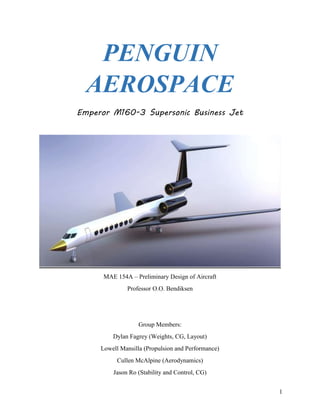
  • 1. 1 PENGUIN AEROSPACE Emperor M160-3 Supersonic Business Jet MAE 154A – Preliminary Design of Aircraft Professor O.O. Bendiksen Group Members: Dylan Fagrey (Weights, CG, Layout) Lowell Mansilla (Propulsion and Performance) Cullen McAlpine (Aerodynamics) Jason Ro (Stability and Control, CG)
  • 3. 3 TABLE OF CONTENTS LIST OF FIGURES 4 LIST OF TABLES 4 INTRODUCTIONS 6 AIRCRAFT LAYOUT AND DESIGN 7 LAYOUT CONSIDERATIONS 7 EXTERIOR LAYOUT 8 INTERIOR LAYOUT 13 CENTER OF GRAVITY 18 AERODYNAMICS 21 PLANFORM SELECTION 21 SUBSONIC AERODYNAMICS 24 Cruise Performance 24 Takeoff and Landing Performance 27 SUPERSONIC AERODYNAMICS 29 Layout and Configuration 29 Cruise Performance 30 PROPULSION AND PERFORMANCE 32 ENGINE SELECTION 32 RATE OF CLIMB 32 ABSOLUTE AND SERVICE CEILING 34 CRUISING AND MAXIMUM MACH NUMBERS 36 STABILITY AND CONTROL 39 CENTER OF GRAVITY 39 AERODYNAMIC CENTER 40 NEUTRAL POINT AND STATIC MARGIN 40 MOMENT COEFFICIENT WITH RESPECT TO ANGLE OF ATTACK 43 TRIM ANALYSIS 43 FUEL MANAGEMENT 46 STRUCTURES AND MATERIALS 47 CONCLUSION 48 RANGE BENEFITS 48 LAYOUT AND CONFIGURATION ERROR! BOOKMARK NOT DEFINED. REFERENCES 50 APPENDIX 51 APPENDIX A: LAYOUT AND CONFIGURATION 51 AIRCRAFT WEIGHT ESTIMATION EQUATIONS 53 APPENDIX B: AERODYNAMICS 55 APPENDIX C: PROPULSION AND PERFORMANCE 60 APPENDIX D: STABILITY AND TRIM 61
  • 4. 4 LIST OF FIGURES Figure 1: Side View 9 Figure 2: Front View 9 Figure 3: Top View 10 Figure 4: Overturn Angle, Main Landing Gear (Sadraey, 2012) 12 Figure 5: Interior Cabin Dimensions 13 Figure 6: Interior Cabin Layout 14 Figure 7: Fuel Tank Locations 16 Figure 8: Transonic Area Plot 17 Figure 9: L/D vs. sweep angle at various Mach numbers 21 Figure 10: Lift coefficient vs. sweep angle for each Mach number 22 Figure 11: Drag coefficient vs. sweep angle at each Mach number 22 Figure 12: Optimized Wing Planform Dimensions 24 Figure 13: Rate of Climb vs. Altitude 34 Figure 14: Available and Required Thrust at Altitudes 35 Figure 15: Trim Plot Subsonic Case 1 Loading Conditions 45 Figure 16: Trim Plot Supersonic Case 1 Loading Conditions 45 Figure 17: Engineering Drawing 52 Figure 18: Maximum Cl Approximations by Nicolai 55 Figure 19: Raymer Table B.1 (continued on next page) 58 Figure 20: Empirical Pitching Moment Factor 63 Figure 21: Downwash Estimation M = 0 64 Figure 22: Subsonic Trim Plots M = .96 66 Figure 23: Supersonic Trim Plots at M = 1.8 68 LIST OF TABLES Table 1: Similar Business Jet Dimensions 7 Table 2: Landing Gear Wheel Track Calculations 12 Table 3: Volumes and Surface Areas 17 Table 4: Interior Cabin Volumes 18 Table 5: Loading Conditions 19 Table 6: Center of Gravity Locations 19 Table 7: CFD Flight Parameters 25 Table 8: Supersonic Interpolation Data 30 Table 9: Rate of Climb 33 Table 10: Absolute and Service Celing 35 Table 11: Induced and Wave Drag Estimations 36 Table 13: Static Margins for Loading Cases 42 Table 14: π‘ͺπ‘΄πœΆ for Loading Cases 43 Table 15: Angle of Attack and Elevator Deflections for Loading Cases 46 Table 16: Weight Breakdown by Component 51
  • 5. 5 Table 17: Iterative CFD Data (continued on next page) 56 Table 18: Rate of Climb at Varying Altitudes 60 Table 19: Weight Distribution Breakdown 61 Table 20: Relevant Stability Coefficients 62 Table 21: Subsonic Loading Conditions at M = .96 65 Table 22: Supersonic Loading Conditions at M = 1.8 67
  • 6. 6 INTRODUCTIONS In a world of growing corporate connections and interdependence, the need for supersonic business travel is growing significantly. While social media and internet related technology can provide some solutions to problems involving long distance business operations, often for general travel, supervising purposes and brokering critical business transactions, physical travel is necessary. For busy CEOs, movie moguls, and other VIPs, time is often even more important than money, and a supersonic business jet could provide a relaxing, efficient, and most importantly, quick method of travel. There are a few popular concepts and current business jets that provide luxury and speed, but few can accomplish both. This report summarizes design considerations for a supersonic business jet based primarily on the Aerion AS2 that would be optimized for both near sonic and supersonic cruise while maintaining a high standard of comfort. The aircraft is designed to transport 8 to 12 executive passengers, including 2 passengers and a flight attendant. The business jet will cruise between 45,000 and 49,000 feet and ideally would have a range of about 4000 nautical miles at a subsonic speed of Mach .93, with the potential for supersonic cruise at Mach 1.8 with a range of 1900 nautical miles; maximum operating speed will be at Mach 1.9. Since FAA regulations do not currently permit supersonic travel over the United States, the designed aircraft would utilize the subsonic cruise specifications over the mainland and accelerate to supersonic speeds outside of the mainland to uphold quick travel requirements. The remainder of the report will describe a baseline design and aircraft layout as well as discuss all aerodynamic, propulsion, performance, and stability calculations that pertain to the required design parameters.
  • 7. 7 AIRCRAFT LAYOUT AND DESIGN Originally we based our aircraft design on the Aerion AS2, using its dimensions and component locations. As we progressed with our calculations for aerodynamics, propulsion, and stability we altered our layout based on functionality while maintaining a certain degree of aesthetics. Layout Considerations To begin the process of designing the Emperor, initial research was conducted of supersonic and high-subsonic business jets in the market to get an idea of the sizing of the fuselage and the dimensions of the passenger cabin. Basic measurements and weights were recorded for aircraft such as the Aerion AS2 supersonic business jet, the Gulfstream G650 and G650ER high- subsonic jets, and other, smaller business jets. The data found was used to size the fuselage of our aircraft accordingly to provide maximum comfort and space for the passengers while also minimizing negative performance effects. This research is compiled in Table 1. Table 1: Similar Business Jet Dimensions Aircraft Length (ft, in) Width (ft, in) Height (ft, in) Cabin Length (ft, in) Cabin Width (ft, in) Cabin Height (ft, in) Aerion AS2 160' 70' 27' 30' 7' 3" 6' 2" Gulfstream G650 99' 9" 99' 7" 25' 8" 53' 7" 8' 6" 6' 5" Gulfstream G650ER 99' 9" 99' 7" 25' 8" 47' 8' 6" 6' 5" Gulfstream G550 96' 5" 93' 6" 25' 10" 43' 11" 7' 5" 6' 2" Bombardier Challenger 650 87' 10" 69' 7" 20' 5" 40' 3" 7' 11" 6' Learjet 75 58' 50' 11" 14' 19' 9" 5' 1" 5' Hawker 800XP 51' 2" 51' 4" 18' 1" 21' 3" 6' 5' 9" As the table shows, the Gulfstream G650 and G650ER have the largest cabin width and standup height in the private business jet class. As a way of ensuring maximum comfort for our passengers, we decided to imitate the interior dimensions of the G650 for our fuselage
  • 8. 8 dimensions, while the exterior dimensions more closely resembled the Aerion AS2 due to the supersonic capability and the need for fuel storage, wing sweep, and other factors. The Emperor’s design predecessor was ultimately the Aerion, as it is the only supersonic business jet that is far along in the design process. Other considerations that were necessary for supersonic performance were also considered, such as highly swept wings and a tapered fuselage section, which will be described in greater detail in the following section. EXTERIOR LAYOUT The fuselage size was an estimate based on the Aerion AS2, and is set to 110 feet from the nose to the back end of the tail cone, while the length from the nose to the end of the tail surfaces is 120 feet. The total wingspan of the Emperor is 98.6 feet, and the total height from landing gear to the tip of the T-tail is 35.4 feet. These dimensions are illustrated below in Figures 1, 2, and 3. Engineering drawings of the Emperor are located in Appendix A. As is best shown in the top view of the Emperor, the fuselage is tapered to attempt to follow the transonic area rule and achieve better supersonic performance. The explanation and area-rule plots are located below, in the Weights, Areas, and Volumes section.
  • 9. 9 Figure 1: Side View Figure 2: Front View 110’ 0” 35’5” 98’ 7” 37’ 4”
  • 10. 10 Figure 3: Top View A 10 foot Von Karman nose cone was also chosen in order to reduce drag while satisfying the FAR requirement of a 15Β° line-of-sight for the pilots on takeoff and landing. The Emperor’s pilots have a 16.07Β° LOS, which eliminates the need for a β€œPinocchio” nose or a droop-nose like that of the Concorde. The Von Karman shape is the conventional nose used on most supersonic fighters due to its ideality at higher Mach numbers. The Emperor uses a low-mounted wing and high T-tail configuration, and the sizings for the lifting bodies are located in the Aerodynamics and Stability Sections. Due to the presence of the two fuselage-mounted engines, a T-tail is required to avoid unwanted downwash effects on the horizontal stabilizers from the engine exhaust. Both the horizontal and vertical tails use a NACA 0012 symmetric airfoil. The tail planform area was determined to be 450 ft2 through stability calculations, and the tail span was determined to be 37.35 feet with an aspect ratio of 3.1, a sweep of 49Β°, and an incidence angle of -2.4Β°. The vertical stabilizer was sized using engine-out estimations discussed in the Stability and Control Section, and was determined to be 14 feet in span with a 0Β° trailing edge sweep. 120’ 0”
  • 11. 11 In order to achieve enough thrust for supercruise, a tri-jet configuration was chosen for the Emperor. Two BruinJet205 low-bypass turbofan engines are mounted on vibration-dampening pylons to the fuselage behind the wings, at a distance of 92 feet from the nose. A third BJ205 is mounted at the top of the fuselage above the tail, and the vertical stabilizer originates from the top surface of that engine. The engines were placed where they are on the Emperor for a variety of reasons. The main reason is that fuselage-mounted engines provide β€œclean” aerodynamics for the wings, meaning that the wing can be optimally designed without having to take into account mounting pylons or the additional weight of the engines on the wing. It also shortens the ground clearance needed, which means that longer, complicated landing gear is not needed to compensate for the wing mounts. Finally, by choosing the fuselage-mounted engines, it allows for a quieter passenger cabin, and is the norm for most business jets on the market today. The main landing gear of the Emperor was placed 79 feet from the nose, at a lateral spacing of 5 feet from the centerline of the aircraft. In order to provide 11Β° of clearance for the takeoff transition distance, the landing gear is set to hydraulically extend to 8 ft below the fuselage. The wheel track of the main gear was determined using the equation involving the overturn angle of the aircraft: π‘Œπ‘‚π‘‡ = 𝐻 𝐢𝐺 tan Ξ¦ 𝑂𝑇 where YOT is the wheel track, HCG is the vertical distance from the runway to the center of gravity of the aircraft, and Ξ¦ 𝑂𝑇 is the overturn angle, as is illustrated in Figure 4.
  • 12. 12 Figure 4: Overturn Angle, Main Landing Gear (Sadraey, 2012) The recommended envelope for the overturn angle is Ξ¦ 𝑂𝑇 β‰₯ 25Β°. Because of the slender fuselage of the Emperor, a conservative overturn angle of 26Β° was chosen, which resulted in a wheel track of 4.66 feet. As 4.66 feet was the minimum wheel track for stable taxiing, it was rounded up to 5 feet for safety. The calculations for HCG as well as the wheel track are located in Table 2. Table 2: Landing Gear Wheel Track Calculations Component CG Height, ft Weight, lbs Forward Engines 11.79 10722.44 Fuselage 10.25 8654.02 Wings 8.00 12754.93 Aft Engine 17.33 5361.22 Horizontal Stabilizers 35.00 1585.92 Vertical Stabilizer 26.00 1036.67 Payload 10.50 3120.00 Systems 8.50 11816.82 Fuel 8.00 64100.00 Total CG Height, ft Overturn Angle, rad Landing Gear Lateral Spacing, ft 9.56 0.45 4.66
  • 13. 13 INTERIOR LAYOUT Figure 5: Interior Cabin Dimensions As shown in Figure 5, the main cabin fuselage has an interior centerline width of 8’2” (allowing for 2” of exterior skin thickness) and has a height of 6’4” to accommodate taller passengers. This allows for 2’ 2” of space under the cabin for controls, wiring, and structural necessities. For the Emperor, we have chosen a sleek and streamlined double-club configuration: on either side of the fuselage are three sets of two seats each, with a table for each set. In order to provide adequate room for passengers to spread out, the cabin has been chosen at a length of 65 feet from the cockpit doors. A full galley and lavatory are also provided on the Emperor, fore and aft of the passenger cabin, respectively. Finally, at the farthest aft in the cabin, is a luggage compartment with a capacity of approximately 230 cubic feet. The configuration of the cabin is outlined below in Figure 6.
  • 14. 14 Figure 6: Interior Cabin Layout An engineering drawing of the interior dimensions is also provided in Appendix A. The seats that we have chosen provide top-of-the line luxury and comfort, at 24” wide and 48” tall, allowing for an approximately 26” aisle in the seating area. At maximum passenger capacity, the Emperor can carry 12 passengers, 1 crew member, and 2 pilots plus 60 lbs of luggage per passenger. WEIGHTS, AREAS, AND VOLUMES Statistical weight estimations were used for each individual component of the aircraft. Using Equations 15.46 - 15.49 and 15.52 - 15.58 from Raymer’s Aircraft Design: A Conceptual Approach, as well as landing gear weight estimations found in Torenbeek’s Synthesis of Subsonic Airplane Design and control systems estimates from Sadraey’s Aircraft Design: A Systems Engineering Approach, the weight of each individual component was calculated and summed to determine the total weight of the Emperor. The weight breakdown is contained in Table 16 in Appendix A: The statistical estimation equations are listed in the Appendix under Aircraft Weight Estimation Equations. In order to compensate for the size of the Emperor and its capabilities, composite materials were used extensively in the construction of our aircraft to reduce weight
  • 15. 15 where needed. Using so-called fudge factors located in the Weight Estimation section in Raymer, the weights of components such as the wings, fuselage, tail surfaces, and engine housings were reduced by factors of 10-20%. This allowed the Emperor to drop a significant amount of structural weight (which could then be replaced with fuel) while remaining under the MTOW conditions for the lifting surfaces and takeoff calculations. The Emperor also uses titanium landing gear in order to reduce weight further. Titanium was chosen due to its high strength-to- weight ratio, and it allowed a reduction in weight from traditional steel landing gear of 43%. The high price of titanium is a non-issue in our case, as it will be negligible compared to the aircraft price. In the Emperor, the fuel is contained within two wing tanks as well as a reinforced tank underneath the fuselage to protect against rupture. The fuel chosen for this aircraft is Jet A-1, with a density of 6.71 lbs/gal. With 64,100 lbs of fuel, there are approximately 9,552 gallons of fuel carried onboard in max range configuration. The wing tanks in the Emperor consist of 70% of the wing volume, for a value of 426.17 ft3 , or 3187.95 gallons per wing, which corresponds to 42782.34 lbs of fuel in the combined wing tanks. The remaining fuel is placed in the fuselage tank, which has a volume of 424.70 ft3 (3177 gal) and a weight of 21317.65 lbs. The fuel was placed under the wings and fuselage in order to avoid a large CG shift as fuel was expended, and also eliminates the need for trim tanks. A fuel pumping plan is discussed in the Stability and Control section. A diagram of the fuel tanks is located below in Figure 7:
  • 16. 16 Figure 7: Fuel Tank Locations Once the aircraft was assembled in SolidWorks, a series of surface area and volume calculations were carried out. Firstly, the cross-sectional area was taken every 5 feet for the entire length of the Emperor for transonic area rule calculations. The plot of these areas is shown in Figure 8, plotted against the Sears-Haack body profile, which is argued to be the ideal drag- reducing area distribution. The Sears-Haack equation for cross sectional area is 𝑆(π‘₯) = πœ‹π‘… π‘šπ‘Žπ‘₯ 2 [4π‘₯(1 βˆ’ π‘₯)] 3 2⁄ . While this profile is impossible to obtain for any type of aircraft, it is considered a template for the cross-sectional area of the aircraft. As the graph on the next page shows, the Emperor’s cross-sectional area is vastly different than the Sears-Haack body. This is due to a number of reasons. The wings on the Emperor are not only very large, but are also highly swept, meaning that the area distribution is weighted towards the back of the aircraft, whereas the Sears-Haack body begins to taper downward at its midpoint. Also, the Emperor has rear-mounted external
  • 17. 17 engines, and each of those adds a significant cross-section to the total profile. In the end, the fuselage was necked down at the wing root wide enough to allow passengers to reach the lavatory and luggage compartment in the aft section of the cabin, but structurally speaking, there would be no way to taper the fuselage enough to make the aircraft more closely resemble the Sears-Haack distribution. Figure 8: Transonic Area Plot In addition, volume and surface area calculations were performed in SolidWorks, and the results (including the total wetted area of the Emperor) are located in Table 3: Table 3: Volumes and Surface Areas Aircraft Component Volume, ft3 Surface Area, ft2 Fuselage 4871.65 3288.03 Wings 1217.62 4590.71 Engines (all three) 1086.12 1164.93 Horizontal Tail 165.79 542.34 Vertical Tail 65.83 224.55 Total for Aircraft 7407.01 9810.56 0 20 40 60 80 100 120 140 160 0 20 40 60 80 100 120 Cross-SectionalArea,ft2 Fuselage Stations, ft Emperor Cross-Sectional Area vs. Sears-Haack Body Distribution Emperor Sears-Haack Wing Tapered Fuselage Forward EnginesFuselage Nose Tail
  • 18. 18 Also, volumes for the interior pressurized cabin were calculated, as the volume of the pressurized cabin had an effect of the fuselage structural weight. These calculations are in Table 4: Table 4: Interior Cabin Volumes Cabin Component Volume, ft3 Cockpit 683.92 Fuselage (Untapered) 2117.96 Tapered Section 879.99 Aft of Tapered Section 353.73 Total Pressurized Volume 4035.60 CENTER OF GRAVITY The center of gravity of the Emperor was determined by applying a moment equilibrium on the aircraft. We estimated the location of each component of the aircraft with respect to a coordinate system located at the nose. Table 19 in Appendix D displays these values as well as the moment that is created by each component about the aircraft's nose. All of the components generate a counterclockwise moment which, under trim conditions, should be counterbalanced by the lift at the aircraft's center of gravity. Under trim, the force of lift is equal to the aircraft’s weight, thus dividing the total moments by the aircraft's weight will equal the distance of the Emperor’s center of gravity from its nose, as well as a percentage of the mean aerodynamic chord. The center of gravity calculation is located below: π‘₯ 𝑐𝑔 = βˆ‘ 𝑀 π‘Šπ‘‘π‘œπ‘‘π‘Žπ‘™ = 76.93 𝑓𝑑 = 51.95 %𝑀𝐴𝐢 An analysis of different loading conditions was considered as well. These loading conditions are outlined in Table 5:
  • 19. 19 Table 5: Loading Conditions Loading Condition Payload Fuel I Max Max II Max Min III Min Max IV Min Min For maximum load, all components will be on board while minimum load will exclude the passengers, luggage, and flight attendant. Similarly, maximum fuel considers fuel tanks to be completely full, while minimum fuel requires that the aircraft retain approximately 20% of the total fuel capacity to allow for landing and remaining in a holding pattern. Applying this methodology, we calculated the CG both from the nose and as a percentage of mean aerodynamic chord for all load conditions considered, found in Table 6. During flight, the CG does not remain constant because fuel is expended, reducing the weight and shifting weight distribution in the wings and fuselage. The leading edge of the MAC was determined to be located 69.36 ft from the nose, so the equation %𝑀𝐴𝐢 = βˆ’(𝑋𝐿𝐸,𝑀𝐴𝐢 βˆ’ 𝑋 𝐢𝐺) 𝑀𝐴𝐢 is used to find the percentage shift in center of gravity. Table 6: Center of Gravity Locations Load Case CG Location from nose, ft CG Location, %MAC CASE I: Max Payload, Max Fuel 76.93 51.95 CASE II: Max Payload, Min Fuel 75.45 41.81 CASE III: Min Payload, Max Fuel 77.52 56.05 CASE IV: Min Payload, Min Fuel 76.41 48.43 These CG shifts are fairly optimistic, as there is not much of a difference in the location of the center of gravity as the Emperor expends fuel. However, this can be explained by the fact that the largest component of the weight in the aircraft, the fuel, is located very close to the center of
  • 20. 20 gravity. This was chosen on purpose to allow for maximum stability as the Emperor burns fuel. This is a very common fuel placement scheme and is used by many aircraft in production and use today. An additional discussion on the center of gravity shifts is located in the Stability and Control section of the report.
  • 21. 21 AERODYNAMICS Planform Selection First and foremost, the wing planform geometry was optimized from the midterm report. This was accomplished by examining the effects of sweep in the transonic region at three new leading edge sweep conditions: 41, 45, and 49 degrees. For each new value for leading edge sweep, a computational Excel sheet was used to determine the trailing edge sweep and tip chord length required to maintain the aspect ratio and root chord length determined in the midterm report to minimize changes to other aspects of the aircraft. Once these values were determined, the CFD code was run for the cases of Mach 0.93 to Mach 1.08 at intervals of 0.03. At each interval, the mesh was altered to reflect each new leading edge sweep and the corresponding plan form conditions. This process provided the following graphs: Figure 9: L/D vs. sweep angle at various Mach numbers 9 11 13 15 17 19 21 23 40 42 44 46 48 50 L/D Sweep Angle L/D vs. Sweep Angle M=0.93 M=0.96 M=0.99 M=1.02 M=1.05 M=1.08
  • 22. 22 Figure 10: Lift coefficient vs. sweep angle for each Mach number Figure 11: Drag coefficient vs. sweep angle at each Mach number Data for these calculations, including percent reduction in various parameters, is presented in Table 15 of Appendix B. While there is a notable reduction in lift coefficient, the reduction in 3.50E-01 3.70E-01 3.90E-01 4.10E-01 4.30E-01 4.50E-01 4.70E-01 4.90E-01 5.10E-01 5.30E-01 5.50E-01 40 42 44 46 48 50 Coefficient Sweep Angle Lift Coefficient vs. Sweep Angle M=0.93 M=0.96 M=0.99 M=1.02 M=1.05 M=1.08 1.50E-02 2.00E-02 2.50E-02 3.00E-02 3.50E-02 4.00E-02 4.50E-02 5.00E-02 40 42 44 46 48 50 Coefficient Sweep Angle Drag Coefficient vs. Sweep Angle M=0.93 M=0.96 M=0.99 M=1.02 M=1.05 M=1.08
  • 23. 23 drag coefficient is more than twice that of lift (even more in supersonic regions), so it was decided that a leading edge sweep of 49 degrees would be adopted to significantly reduce drag. Once the plan form was officially selected, the following calculations could be made; where A is aspect ratio, b is wingspan, S is wing area, and cr and ct are the chord length at the root and tip respectively. Our aspect ratio is given by 𝐴 = 𝑏2 𝑆 = 7.20 Therefore we can determine the wingspan to be 𝑏 = βˆšπ΄π‘† 2 β‰ˆ 98.6 𝑓𝑑. Similar to the specifications for the midterm report, we maintained that the chord at wing root would be 𝑏 2 = 2.5 𝑐 π‘Ÿ As a result, the wing root chord length is 𝑐 π‘Ÿ = 𝑏 2 βˆ— 2.5 = 98.6 2 βˆ— 2.5 β‰ˆ 19.72 𝑓𝑑. In addition, the geometry based on the effects of wing sweep at transonic Mach numbers dictates that the ratio of the tip chord length to the root chord length be: πœ† = 𝑐𝑑 𝑐 π‘Ÿ = .390 Thus, it can be shown that the tip chord would be 7.66 ft.
  • 24. 24 Figure 12: Optimized Wing Planform Dimensions SUBSONIC AERODYNAMICS Cruise Performance A preliminary analysis was used to determine the achievable range of the plane. First, an approximation was made with the assumption that if the range can be accomplished at cruise, then other factors such as climb and descent can be modified from the preliminary analysis. To calculate the range that can be achieved in nautical miles, the Breguet range equation will be used, where a final conversion to nautical miles will be made at the end. Note that in this equation, the velocity used is assumed to be the given cruise velocity of Mach .96, which is an average of the range of prescribed Mach numbers in the requirements. From Table B.1 in Raymer’s Aircraft Design, the cruise altitude of 41000 feet corresponds to a speed of sound a = 968.1 fps. With the velocity at cruise determined, the Reynolds number can
  • 25. 25 be found using the equation, 𝑅𝑒 = πœŒπ‘‰π· πœ‡ , where the density and viscosity of air were determined from altitude tables and the characteristic length D is the mean aerodynamic chord. This gave us a subsonic cruise Reynolds number of just over 24 million. Thus, the velocity that will be used is V = Ma = (968.1 fps)*(.96) = 929.37 fps. The assumption that trim flight equates weight and lift yields the equation, 𝐿 = π‘Š = π‘žπ‘†πΆπ‘™, where q is the dynamic pressure, S is our wing planform area, and Cl would be the coefficient of lift. Trim flight cruise conditions dictate the dynamic pressure with the wing planform area being set in the Planform Selection Section of this report, and thus, we can find the Cl of our plane during cruise trim conditions. The following equation shows this analysis: 𝐢𝑙 = π‘Š π‘žπ‘† = 123000 (241.847)(1350) = 0.376 From this calculation of Cl, the given CFD code was used to iterate angles of attack with the selected planform until the Cl approached the value required for trim. It was found that a subsonic cruise of Mach 0.96 yielded a Cl of 0.372 at an angle of attack of 4 degrees. While this is slightly lower than trim conditions, due to the iterative nature of the CFD calculations, for the time constraints of this project it was concluded that the result was satisfactory. The following table shows the results obtained from the CFD program. Table 7: CFD Flight Parameters Ξ± Cd, i+w CM,cr/4 𝐿 𝐷 𝑖+𝑀 𝐢𝐿 𝛼,π‘Žπ‘£π‘”. X%mac@CM=0 4 0.017 -0.66 20.97 5.33 45.94
  • 26. 26 Using these parameters and trim conditions, it was determined that induced and wave drag on the wing at subsonic trim is Di+w = 5550.4 lbs. In order to find the parasitic drag at subsonic conditions, the following equations, dependent on wetted area, reference area, and skin coefficient, are used: 𝐢 𝐷 𝑃 = 𝐢𝑓 𝑆 𝑀𝑒𝑑 π‘†π‘Ÿπ‘’π‘“ = (.00247)(3424.218) (2735) = .00310 𝐢𝑓,π‘ π‘’π‘π‘ π‘œπ‘›π‘–π‘ = . 074 𝑅𝑒.2 β‰ˆ .00247 𝑅𝑒 = πœŒπ‘‰ ( 𝑐𝑑 + 𝑐 π‘Ÿ 2 ) πœ‡ = (.00056)(929.376)( 7.66 + 19.72 2 ) 2.97 βˆ— 10βˆ’7 = 2.4 βˆ— 107 Utilizing the relevant parameters at Mach 0.96, the parasitic drag coefficient (𝐢 𝐷 𝑝 ) was determined to be .0031. Combining the parasitic and induced/wave drag coefficients, our total drag was found to be D = 6,561.2 lbs. at subsonic cruise. We calculated range using 𝑅 = ( 𝑉 𝑐𝑑 ) ( 𝐿 𝐷 ) ln ( π‘Š0 π‘Šπ‘– ) where lift can be set equal to weight (since the aircraft is at trim), the velocity is constrained by the Mach number, and the tip chord is provided as discussed in the plan form selection section. Weights were discussed in the layout section, and were determined by estimates provided in Raymer. Despite numerous iterations of the CFD code, in order to obtain sufficient lift to maintain level flight at trim, the minimum induced drag was found to be insufficient to allow for a range of 4500 nmi as requested in the design specifications. While the induced drag was successfully minimized, the maximum range possible for our aircraft was found to be R = 3970 nmi.
  • 27. 27 Takeoff and Landing Performance Takeoff performance is a vital aspect of subsonic aerodynamics. If the plane cannot takeoff, then the plane cannot fly. The prescribed runway length was given to be no more than 6000 ft. As a result, our plane must be sized such that this take off length is possible. Total takeoff distance required is determined through the sum of the ground roll distance, rotation distance, transition distance, and climb out distance: π‘†π‘‘π‘œπ‘‘π‘Žπ‘™ = 𝑆 𝐺 + 𝑆 𝑅 + 𝑆 𝑇𝑅 + 𝑆 𝐢𝐿. First and foremost, the stall speed at sea level must be determined in order to approximate takeoff speed. Figure 13 in Appendix A taken from the Nicolai Aircraft Design book with our planform was used to determine CL,max. Takeoff speed is defined as 1.2 times the stall speed, which can be found by using CL,max of our wing from the figure at sea level. 𝑉𝐿𝑂𝐹 = 1.2𝑉𝑠 = 1.2√ π‘Š πœŒπ‘ π‘’π‘Ž 𝐢𝑙,π‘šπ‘Žπ‘₯ 𝑆 𝑀 = 1.2 √ 123000 𝑙𝑏𝑓. (.00238 𝑠𝑙𝑒𝑔𝑠 𝑓𝑑3 )(1.35)(1350 𝑓𝑑2) = 285.776 𝑓𝑑. π‘ βˆ’1 The ground roll distance then becomes: 𝑆 𝐺 = 1 2 π‘€π‘Žπ‘ π‘  βˆ— 𝑉𝐿𝑂𝐹 2 𝑇𝑒| 𝑉 𝐿𝑂𝐹/√2 = 2163.592 𝑓𝑑. Where 𝑇𝑒 = 𝑇 βˆ’ 𝐷 βˆ’ πœ‡(π‘Š βˆ’ 𝐿) There is also a rotation distance in which the plane begins to rotate to an angle that is necessary to clear an obstacle of said amount of height. This is defined as the time it takes to rotate the aircraft to an angle of attack such that a lift coefficient of 0.8CL,max is generated1 . Since 1 Taken from Bendiksen’s Lecture Notes Chapter 2: Aircraft Performance eq. 2.159
  • 28. 28 there is no specific way estimate that time, we arbitrarily assigned a value of 2 seconds for this period. 𝑆 𝑅 = 𝑉𝐿𝑂𝐹 𝑑 𝑅 = 571.553 𝑓𝑑. After rotation, the plane has β€œtaken off” and begins to fly along an arc until the climb angle Ξ³cl is reached. This expression is defined as: sin 𝛾 𝐢𝐿 = 𝑇 βˆ’ 𝐷 π‘Š And the transition distance is shown to be equivalent to: 𝑆 𝑇𝑅 = 𝑅 sin 𝛾 𝐢𝐿 = 3230.739 𝑓𝑑. where 𝑅 = 𝑉𝐿𝑂𝐹 2 0.152𝑔 There is also a climb out distance if the obstacle is taller than the plane’s altitude by the end of the transition run, which is not applicable in this situation, but is defined as: 𝑆 𝐢𝐿 = β„Ž βˆ’ 𝑅 (1 βˆ’ cos 𝛾 𝐢𝐿) tan 𝛾 𝐢𝐿 Therefore, our total takeoff distance given a 35 foot clearance at the end of the run comes out to be 5965.885 feet. This value accounts for the total drag coefficient which includes parasitic and wing drag. Attention was given to the rotation angle, which is approximately 11 degrees, in order to ensure that there are no tail strikes at the end of the rotation run. Another final property to note, is the requirement that throttle be at 75% for takeoff distance to not exceed runway allotted. This is unfortunately due to excess thrust from the engine scaling as detailed in the Propulsion Section. Too much thrust eventually causes the transition distance to increase at a faster rate than ground roll decreases.
  • 29. 29 Landing is essentially the opposite of takeoff. Using a combination of equations from Raymer’s Aircraft Design: A Conceptual Approach and Bendiksen’s Lecture Notes, the entire distance for landing is calculated through the sum of flare, braking, and ground roll distance. Since our climb-out height is higher than the obstacle, we do not need to worry about approach distance. Flare speed is defined as: 𝑉𝑓 = 1.23 βˆ— 𝑉𝑠 = 1.23√ π‘Šπ‘“ πœŒπΆπ‘™ 𝑆 = 1.23√ 71720 (.00238)(1.35)(1350 = 223.675 𝑓𝑑. Touchdown speed can be calculated similarly using 1.3 times the stall speed, which comes out to be 236.41 feet. 𝑠𝑓 = 𝑅 sin 𝛾 = 𝑇 βˆ’ 𝐷 π‘Š 𝑉𝑓 2 . 152𝑔 = 3452.262 𝑓𝑑. Braking distance is a function of touchdown speed and delay, which we assumed to be 2 seconds once again due to size of the aircraft: 𝑠 π‘π‘Ÿ = 𝑉𝑇𝐷 𝑑 = 472.809 𝑓𝑑. Finally the same equation used for ground roll before is evaluated using the new touchdown speed, yielding sg = 844.581 ft. Total ground distance is found to be 4769.65 feet. SUPERSONIC AERODYNAMICS Layout and Configuration To accommodate supersonic cruising conditions, a variety of factors were employed in the layout design and configuration of the plane. First of all, an aggressive wing sweep as proposed in the Planform Selection Section will help reduce the perpendicular area as seen by the airflow, and thus, reduce the supersonic drag. Since our operating speeds lie within the transonic and supersonic region, the transonic area rule is utilized, which states that any cross sectional area to the airflow must be smooth to reduce drag. Abiding by that rule, the fuselage has been necked
  • 30. 30 down near the wing attachment areas. In addition, the nose of the plane uses a less pronounced von Karman cone in order to reduce the amount of drag from the nose of the fuselage. Cruise Performance Using a method similar to that used in the Subsonic Cruise Performance section, the supersonic drag on the plane can be determined. First and foremost, the Cl,max must be determined for trim cruise conditions at high Mach numbers. Once again using Table B.1 from the Raymer book, we can determine the speed of sound and air density at 41000 feet to be 968.1 fps and .00056 slugs/ft3 respectively. Our cruise velocity thus corresponds to 𝑉 = π‘€π‘Ž = (1.8)(968.1) = 1742.58 𝑓𝑝𝑠. With these numbers, we can determine that our dynamic pressure q = 850.243 lb/ft.2 . Below, the calculations are shown for the determination of Cl,max at the cruise altitude: 𝐢𝑙,π‘šπ‘Žπ‘₯ = √ π‘Š π‘žπ‘† = √ 123000 (850.243)(1350) = .10716 Once again, an iterative methodology was conducted to find a satisfactory Cl for the above conditions. Since supersonic flight cannot be achieved legally in US airspace, flight conditions for Mach 1.8 would be slightly different from that of subsonic speeds. The assumption was made for a significant loss of fuel due to cruising at subsonic speed. Thus, a Cl = .0958 was deemed satisfactory and within the bounds of error. The table below summarizes the data extrapolated from the CFD output results for this new angle of attack and cruise condition. Table 8: Supersonic Interpolation Data Ξ± Cd, i+w CM,cr/4 𝐿 𝐷 𝑖+𝑀 𝐢𝐿 𝛼,π‘Žπ‘£π‘”. X%mac@CM=0 2 0.0197 -0.183 4.866 2.743 57.229
  • 31. 31 To find the parasitic drag at supersonic conditions, the following equations, dependent on wetted area, reference area, and skin coefficient, are used: 𝐢 𝐷 𝑃 = 𝐢𝑓 𝑆 𝑀𝑒𝑑 π‘†π‘Ÿπ‘’π‘“ = (.00186)(3424.218) 2735 . 00233 𝑅𝑒 = πœŒπ‘‰ ( 𝑐𝑑 + 𝑐 π‘Ÿ 2 ) πœ‡ β‰ˆ 4.5 βˆ— 107 𝐢𝑓,π‘ π‘’π‘π‘’π‘Ÿπ‘ π‘œπ‘›π‘–π‘ = 0.455/((log10 𝑅𝑒)2.58 (1 + 0.144𝑀2)0.65) = . 455 (log10 4.5 βˆ— 107)2.58(1 + .144(1.82)) .65 = .00186 Note the similarities in this process and the one conducted in the Subsonic Cruise Performance section. With these calculations made, the total drag, accounting for both induced and parasitic, at supersonic trim conditions is 25,285 lbs. If a full tank of fuel was accounted for, then a range of 1900 nautical miles can be reached at this condition.
  • 32. 32 PROPULSION AND PERFORMANCE Engine Selection We used three BruinJet BJ205 engines as the bases for our propulsion and performance analysis with a given SLSD static thrust rating of 20,518 lbs for each engine, thus providing a total SLSD static thrust of 61,554 lbs. From the subsonic and supersonic performance sections, we have found that CD, subsonic = 0.02010 and CD, supersonic = 0.02203. After thorough drag calculations that will be carried out in this section, we have found that the three BJ205 engines cannot provide enough thrust to fly supersonically at both the cruising speed and at the maximum operating speed especially because the available thrust decreases drastically with altitude and speed. To compensate for this discrepancy, we chose to scale up the engines to provide 163.1% more thrust which requires a 128% increase in the diameter of each engine. This increases the overall drag of the aircraft, however, an increase in the amount of thrust available is necessary to fly at high Mach numbers. After scaling the engine to meet drag requirements, we have a new SLSD static thrust rating of 100,394.57 lbs. Rate of Climb At sea-level conditions on a standard day, the aircraft must be able to climb at a rate of 3500 fpm with the maximum gross weight. We can solve for the steady rate of climb using the following formula: 𝑅𝐢 = (𝑇 π΄π‘‰βˆ’π‘‡ π‘…π‘’π‘žπ‘‘)𝑉 π‘Š = √ 2π‘Š πœŒπ‘†πΆ 𝐿 ( 𝑇 𝐴𝑉 π‘Š βˆ’ 𝐢 𝐷 𝐢 𝐿 ) TReqd must be found by equating it to the drag at SLSD. In order to meet realistic and safe standards, 50% engine throttle was used at SLSD conditions to yield the following data:
  • 33. 33 Table 9: Rate of Climb W (lbs) 122,976.35 TAV (lbs) 38,268.85 V (fps) 428.72 TReqd (lbs) 5,927.64 RC (fps) 112.75 RC (fpm) 6765 According to our calculations, the jet will be able to fly at roughly 6765 fpm at 50% throttle, which is well above 3500 fpm at SLSD conditions and maximum gross weight. This is naturally high because the engines must be able to provide enough thrust to fly supersonically, so the amount of available thrust greatly exceeds required thrust. To find the time it will take to reach 37,000 feet, we need to account for the change in thrust and density with increasing altitude. We can approximate rate of climb values at certain points during the ascent and then take the average rate of climb to find the estimated time to reach 37,000 feet. Again, we will perform this at 50% throttle. These calculations are shown in Appendix C. From standard sea level to an altitude of 40,000 feet, the average value of the rate of climb is approximately RCavg = 4141.96 fpm. Dividing this value from 37,000 feet, we get the time it takes to reach that altitude: 𝑑37,000𝑓𝑑 = 37000 𝑓𝑒𝑒𝑑 4243.11 𝑓𝑒𝑒𝑑 min = 8.93 π‘šπ‘–π‘› It will take about 9 minutes to reach an altitude of 37,000 feet, which is under the maximum requirement of 20 minutes. This calculation was performed by using the TSFC to approximate the amount of fuel burned in 5000-foot intervals of altitude. The required amount of thrust at each altitude was equated to the amount of drag using the true airspeed at that altitude and CD, subsonic = 0.02010.
  • 34. 34 Absolute and Service Ceiling The absolute ceiling is the uppermost altitude that the aircraft can theoretically attain, or alternatively, the altitude at which rate of climb hits zero. However, aircrafts never can reach the absolute ceiling, but instead, use the service ceiling as the maximum achievable altitude. For jets, the service ceiling is the altitude at which rate of climb is 500 fpm. We can approximate both the absolute ceiling and the service ceiling by plotting rate of climb versus altitude. We can also plot required thrust and available thrust versus altitude and see that the two theoretically converge. Figure 13: Rate of Climb vs. Altitude 0 1000 2000 3000 4000 5000 6000 7000 0 10000 20000 30000 40000 50000 60000 RateofClimb(fpm) Altitude (feet) Rate of Climb vs. Altitude
  • 35. 35 Figure 14: Available and Required Thrust at Altitudes We approximated the trend between rate of climb and altitude to be linear, producing a relatively strong correlation coefficient of R2 = 0.986. Using the trendline, we can obtain both the absolute ceiling (RC = 0 fpm) and the service ceiling (RC = 500 fpm). Table 10: Absolute and Service Celing Absolute Ceiling 55,900 feet Service Ceiling 54,100 feet The minimum service ceiling is 51,000 feet, so our design clearly meets that expectation. We have assumed full throttle to make ceiling calculations. In addition, we have assumed that once the aircraft hits Mach 0.6 at an altitude of about 20,000 feet, it maintains that Mach number for the rest of the climb. 0 10000 20000 30000 40000 50000 60000 70000 80000 0 10000 20000 30000 40000 50000 60000 Available/RequiredThrust(lbs) Altitude (feet) Available and Required Thrust vs. Altitude Available Thrust Required Thrust
  • 36. 36 Cruising and Maximum Mach Numbers The specified cruise Mach numbers are 0.90-0.95 for subsonic and 1.6-1.8 for supersonic. The maximum operating Mach number is 1.9. To find the required thrust from our engines, we need to find the drag at steady flight conditions: π‘‡π‘…π‘’π‘žπ‘‘ = 𝐷 = 1 2 πœŒπ‘£2 𝐢 𝐷 𝑆 We can approximate total drag by splitting it up into three components: induced, wave, and parasite. Induced and wave drag coefficients can be interpolated from the CFD calculations: Table 11: Induced and Wave Drag Estimations Subsonic (Mach 0.96) Supersonic (Mach 1.8) Maximum (Mach 1.9) V (ft/s) 929.38 1,742.58 1839.39 q (lb/ft2) 241.85 850.24 947.34 CL 0.37673 0.10716 0.09618 CD i+w 0.01700 0.01970 0.01950 Di+w (lbs) 5,550.39 22,612.23 24,938.71 It is clear from the table above that the thrust required will be dictated by the high amounts of drag in supersonic cruising. Additionally, parasite drag also increases with speed. To estimate parasite drag, we will take into account skin-friction effects since it comprises most of parasite drag. Our approximation of parasite drag takes the following form: 𝐢 𝐷 𝑃 = 𝐢𝑓 𝑆 𝑀𝑒𝑑 π‘†π‘Ÿπ‘’π‘“ 𝐢𝑓,π‘ π‘’π‘π‘ π‘œπ‘›π‘–π‘ = 0.074 𝑅𝑒0.2 𝐢𝑓,π‘ π‘’π‘π‘’π‘Ÿπ‘ π‘œπ‘›π‘–π‘ = 0.455/((log10 𝑅𝑒)2.58 (1 + 0.144𝑀2)0.65) ,
  • 37. 37 𝑅𝑒 = πœŒπ‘‰ ( 𝑐𝑑 + 𝑐 π‘Ÿ 2 ) πœ‡ From the Aerodynamic sections, a detailed analysis on drag gives us the following information on parasite drag: Subsonic (Mach 0.96) Supersonic (Mach 1.8) Maximum (Mach 1.9) V (ft/s) 929.38 1,742.58 1839.39 Re 2.400 x 10⁷ 4.500 x 10⁷ 4.750 x 10⁷ Cf 0.00247 0.00186 0.00180 CDp 0.00310 0.00233 0.00226 Dp (lbs) 1,010.80 2,673.49 2,887.59 Like we predicted, the parasite drag increases with Mach number. Now that we have found the parasite, induced, and wave drags, we can find the total drag and compare it to the available thrust of three BJ205 engines at cruising altitude: Subsonic (Mach 0.96) Supersonic (Mach 1.8) Maximum (Mach 1.9) Di+w (lbs) 5,550.39 22,612.23 24,938.71 Dp (lbs) 1,010.80 2,673.49 2,887.59 DTOT (lbs) 6,561.19 25,285.72 27,826.30 TBJ205 @ cruise per engine (lbs) 7,112.79 9,420.66 9,275.50 TAV @ cruise with 3 engines (lbs) 21,338.37 28,261.97 27,826.49 A summary of the required thrusts at each cruising altitude along with the available thrusts using the current engine configuration is shown: Subsonic (Mach 0.96) Supersonic (Mach 1.8) Maximum (Mach 1.9) Required Thrust @ Cruise (lbs) 6,561.19 25,285.72 27,826.30 Available Thrust @ cruise (lbs) 21,338.37 28,261.97 27,826.49
  • 38. 38 We notice that with our engine specifications, we just have enough thrust to cruise at the maximum operating Mach number of 1.9. Although the numbers are dangerously close at Mach 1.9, the aircraft is not designed to fly and cruise at this altitude. At the maximum supersonic cruising speed of Mach 1.8, we have 10% more available thrust than required thrust, therefore we are safe to cruise at these conditions. We have no problems cruising at subsonic speeds.
  • 39. 39 STABILITY AND CONTROL Revisions Several changes in terms of stability were made when the wings and layout were altered. Some components were rearranged in order to control the shift in the center of gravity and the location of the neutral point. Furthermore, many changes were applied to the tail to ensure stability. The conversion to a T-tail significantly affected the effect of downwash on the tail, and a tail incidence angle was introduced to attain proper trim conditions. Lastly, due to issues of controllability, a fuel management outline, which is discussed later, was created to help balance stability and maneuverability. A critical component in aircraft design is stability: determining how well the aircraft can be controlled. Numerous factors contribute to aircraft stability, thus we analyze four different load conditions during for subsonic and supersonic trimmed flight, as was outlined in the Layout Section above. Because our supersonic jet is relying on manual flight controls rather than an electronic interface, we require our jet to have positive stability during trim conditions. The analysis shown will only consider longitudinal stability and all calculations shown will be for the first load case during subsonic and supersonic flight. Stable pitch is determined by two calculations: a positive static margin and a negative moment coefficient with respect to angle of attack (CMΞ±). Center of Gravity The stability of the aircraft is highly dependent on the location of its center of gravity. The procedure for calculating the aircraft’s CG was described earlier in the report. Applying that methodology, we calculated the CG for all load conditions being considered. During flight, the CG does not remain constant as fuel is expended. It was essential to keep the center of gravity from shifting drastically in order to keep the aircraft controllable. We aimed to keep our CG
  • 40. 40 shifts to within 2 ft. between our max fuel and min fuel loading conditions. The table of CG locations was shown in the Layout Section. According to the table, the maximum shift between the loading conditions is approximately 1.48 ft. which meets our goal. However, it is necessary to reiterate from earlier that the weights used were estimated base on specs from other aircraft components, specifically existing business jets, and equations from the textbook Aircraft Design: A Conceptual Approach. We realize that our estimates will carry some degree of error. Aerodynamic Center Similarly to an aircraft's center of gravity, the aerodynamic center of the wing and tail does not stay constant during flight and are critical values in calculating stability. In general, most airfoils have an aerodynamic center at the quarter-chord during subsonic flight but shifts to approximately 45% of the mean aerodynamic chord during supersonic flight. However, utilizing the CFD code we were able to find more realistic values for our wing and tail. We found that the wing’s aerodynamic center is located approximately 38% MAC for low subsonic flight, 45.95% MAC for subsonic cruise, and 57.23% MAC for supersonic cruise, leading to a total AC change of 21.23%. Similarly, the tail’s aerodynamic center moves from 34.56% MAC to 53.23% MAC between subsonic and supersonic conditions. This shift in AC is the result of the wing and tail planform used. For comparison, a delta wing is beneficial for supersonic flight because it would minimize this AC shift. Neutral Point and Static Margin All aircraft have a center of gravity located at a point where there are no pitching moments, regardless of angle of attack. This point is the aircraft's neutral point, or neutral stability, and is the furthest CG location before the aircraft becomes unstable. The equation below was used to
  • 41. 41 locate the neutral point in our business jet, which is expressed as a percentage of the mean aerodynamic chord. π‘₯ 𝑛𝑝 = 𝐢𝐿 𝛼 π‘₯ 𝐴𝐢,𝑀𝑖𝑛𝑔 βˆ’ 𝐢 𝑀 𝛼,π‘“π‘’π‘ π‘’π‘™π‘Žπ‘”π‘’ + πœ‚β„Ž 𝑆𝑑 𝑆 π‘Š 𝐢𝐿 𝛼,π‘‘π‘Žπ‘–π‘™ π‘₯ 𝐴𝐢,π‘‘π‘Žπ‘–π‘™ (1 βˆ’ πœ•πœ– πœ•π›Ό ) + 𝐹𝑝 𝛼 π‘žπ‘† 𝑀 (1 βˆ’ πœ•πœ– πœ•π›Ό )π‘₯ 𝑝 𝐢𝐿 𝛼 + πœ‚β„Ž 𝑆𝑑 𝑆 𝑀 𝐢𝐿 𝛼 (1 βˆ’ πœ•πœ– πœ•π›Ό ) + 𝐹𝑝 𝛼 π‘žπ‘† 𝑀 Several assumptions were made when using this equation. The last term in the numerator and denominator was neglected. According to Raymer, this term is typically ignored in the calculation and is accounted for at the end with test data from similar aircrafts, usually a reduction of the static margin by 1-3% for jets. While acceptable for subsonic flights, this assumption would not be nearly as accurate for supersonic cases. Due to the scarcity of existing supersonic business jets, more research will need to be done in order to account for the reduction in stability in the supersonic flight regime. Besides the force term, other factors, such as downwash effect, πœ‚β„Ž, and moment coefficient for the fuselage were either given or calculated based off estimates from graphs in the textbook. Below are the equations needed to solve for the neutral point. Downwash: Subsonic: πœ•πœ– πœ•π›Ό = ( πœ•πœ– πœ•π›Ό 𝑀=0 ) ( 𝐢 𝐿 𝛼 𝐢 𝐿 𝛼 𝑀=0 ) Supersonic: πœ•πœ– πœ•π›Ό = 1.62𝐢 𝐿 𝛼 πœ‹π΄ Fuselage Pitching Moment 𝐢 𝑀 𝛼 π‘“π‘’π‘ π‘’π‘™π‘Žπ‘”π‘’ = 𝐾 π‘“π‘’π‘ π‘’π‘™π‘Žπ‘”π‘’ π‘Šπ‘“ 2 𝐿 𝑓 𝑐𝑆 𝑀 where Wf = width of the fuselage Kf = empirical pitching-moment factor Lf = length of fuselage A sample calculation is for Case 1 subsonic loading configuration is carried out in Appendix B.
  • 42. 42 The static margin is the difference between the neutral point and the CG location. In order to be stable in flight, the CG of the plane must be ahead of the neutral point. Thus static margin can be expressed as the equation below. π‘†π‘‘π‘Žπ‘‘π‘–π‘ π‘€π‘Žπ‘Ÿπ‘”π‘–π‘› = π‘₯ 𝑛𝑝 βˆ’ π‘₯ 𝐢𝐺 Static margin is normally given as a percent and must be positive for the aircraft to be stable. It is worth noting that too much stability reduces maneuverability. In other words, too stable aircraft are uncontrollable since the pilot cannot not move from one trim condition to another. Typical transport aircraft have a positive static margin of 5-10%, however since our aircraft’s flight envelope includes supersonic conditions, compromises in terms of wing design and performance have significant impacts on stability. The static margin for all load cases as well is shown in the table below. Table 12: Static Margins for Loading Cases Load Case Low subsonic M=0.33 Cruise Subsonic M=0.96 Cruise Supersonic M=1.8 I 14.03% 19.57% 43.76% II 24.18% 29.71% 53.91% III 9.98% 15.52% 39.71% IV 17.56% 23.10% 47.29% Several things can be drawn from the values shown. The low subsonic column was placed in to show that out plane is stable for lower speeds. The Mach number used was estimated to be the speed of the plane after takeoff once all slats and flaps are retracted. All of the values in the table are positive, thus the aircraft remains stable throughout its flight, however the static margin drastically increases as Mach number increases. The largest contributors to this increase are the
  • 43. 43 placement of the wing and tail, the amount their AC shifts, reducing downwash, and the changes in the lift-curve slopes. The high static margins during cruise conditions are not a critical issue since as a transportation jet, maneuverability during cruise is not a priority. Moment Coefficient with Respect to Angle of Attack The second criteria is to have a moment coefficient that opposes changes to angle of attack. This pitching moment derivative is the moment coefficient with respect to angle of attack. It is directly linked to the static margin by the equation below, along with the calculation results for all load cases. 𝐢 𝑀 𝛼 = βˆ’πΆπΏ 𝛼 (𝑋 𝑛𝑝 βˆ’ 𝑋 𝐢𝐺) Table 13: π‘ͺ π‘΄πœΆ for Loading Cases Loading Condition Low subsonic Subsonic Cruise Supersonic Cruise I -0.54551 -1.04401 -1.18741 II -0.94001 -1.58541 -1.46271 III -0.38801 -0.82791 -1.07751 IV -0.68271 -1.23231 -1.28321 As shown, as long as the lift curve slope is positive, the values will show the same conclusions drawn from the static margin calculations. Trim Analysis Enough information has been collected to determine what angle of attack and elevator deflection angle is needed to maintain trimmed flight. We started with moment coefficient about the CG and the total lift coefficient.
  • 44. 44 𝐢 𝑀 𝑐𝑔 = 𝐢𝐿(𝑋𝑐𝑔 βˆ’ 𝑋 π‘Žπ‘π‘€) + 𝐢 𝑀 𝑀 + 𝐢 𝑀 𝑀𝛿𝑓 𝛿𝑓 + 𝐢 𝑀 𝑓𝑒𝑠 βˆ’ πœ‚β„Ž 𝑆𝑑 𝑆 𝑀 𝐢𝐿 𝑑 (𝑋 π‘Žπ‘π‘‘ βˆ’ 𝑋𝑐𝑔) βˆ’ 𝑇 π‘žπ‘† 𝑀 𝑍𝑑 + 𝐷 π‘žπ‘† 𝑀 𝑍𝑑 + 𝐹𝑝 𝛼 π‘žπ‘† 𝑀 (𝑋𝑐𝑔 βˆ’ 𝑋 𝑝) 𝐢𝐿 π‘‡π‘œπ‘‘π‘Žπ‘™ = 𝐢𝐿 𝛼 [𝛼 + 𝑖 𝑀] + πœ‚β„Ž 𝑆𝑑 𝑆 𝑀 𝐢𝐿 𝑑 The goal is to set the moment coefficient in terms of 𝛼 and 𝛿 𝑒. Several assumptions were made to reduce this equation. The last term was neglected for the same reason explained above for the neutral point. The moment coefficient and the drag component from the wing were neglected due to their insignificant contribution to the overall moment. Flaps are not being used during trim conditions. The tail lift coefficient can be found using eq. 16.32 from the textbook. 𝐢𝐿 𝑑 = 𝐢𝐿 𝛼𝑑 [(𝛼 + 𝑖 𝑀)(1 βˆ’ πœ•πœ– πœ•π›Ό ) + (𝑖 𝑀 βˆ’ 𝑖 𝑑) βˆ’ 𝛼0 𝐿 𝑑] The incidence angle on the wing set to zero while tail incidence is at -2.4ΒΊ. The last term in the tail lift coefficient equation can be approximated using eq. 16.18 and Fig. 16.6 from the textbook assuming an elevator area 20% of the tail area. Combining these equations and using the values from the first load case for subsonic and supersonic trim, we get the equations below. Subsonic: 𝐢 𝑀 𝑐𝑔 = βˆ’1.46847𝛼 βˆ’ 0.417307𝛿 𝑒 + 0.099331 𝐢𝐿 π‘‡π‘œπ‘‘π‘Žπ‘™ = 6.50711𝛼 + 0.180100𝛿 𝑒 βˆ’ 0.064570 Supersonic: 𝐢 𝑀 𝑐𝑔 = βˆ’1.46766𝛼 βˆ’ 0.227976𝛿 𝑒 + 0.064467 𝐢𝐿 π‘‡π‘œπ‘‘π‘Žπ‘™ = 3.31761𝛼 + 0.092873𝛿 𝑒 βˆ’ 0.033297 Next, we set different values for the angle of attack and elevator deflection to solve for the coefficients and plotted them to show graphically how they change. Below are the subsonic and supersonic graphs for Case I.
  • 45. 45 Figure 15: Trim Plot Subsonic Case 1 Loading Conditions Figure 16: Trim Plot Supersonic Case 1 Loading Conditions During trimmed flight, the moment about the CG should equal zero. Based on the graph, we see several conditions where the aircraft can trim. According to the CFD calculations, during subsonic and supersonic cruise our 𝐢𝐿 trim is 0.3767 and 0.1072 respectively. In order to meet those conditions, we need to apply approximately 2ΒΊ elevator deflection at an Ξ± of 3ΒΊ for subsonic -0.25 -0.20 -0.15 -0.10 -0.05 0.00 0.05 0.10 0.15 0.20 -0.20 0.00 0.20 0.40 0.60 0.80 1.00 1.20 MomentCoefficient Lift Coefficient Trim Plot Subsonic Case I 4 degrees 2 degrees 0 degrees -2 degrees -4 degrees -6 degrees -8 degrees -0.25 -0.20 -0.15 -0.10 -0.05 0.00 0.05 0.10 0.15 -0.10 0.00 0.10 0.20 0.30 0.40 0.50 0.60 MomentCoefficient Lift Coefficient Trim Plot Supersonic Case I 4 degrees 2 degrees 0 degrees -2 degrees -4 degrees -6 degrees
  • 46. 46 and zero deflection at an Ξ± of 2ΒΊ for supersonic. The table below shows approximated elevator deflections and Ξ± needed to maintain trim. All data tables and graphs for each of the loading conditions are shown in Appendix D. Table 14: Angle of Attack and Elevator Deflections for Loading Cases Subsonic Angle of Attack (deg) Elevator Deflection (deg) Case I 3 2 Case II 3.6 -4 Case III 3.6 4 Case IV 3.9 -1.7 Supersonic Case I 2.1 0 Case II 2.2 -2 Case III 2 2 Case IV 2 0 Fuel Management One issue regarding the over-stability while flying at low Mach numbers must be addressed. As seen in the static margin section, load case II displays a very high static margin. This type of scenario would typically be associated with the aircraft arriving at its destination and needing to land, making controllability a major concern. When experimenting with fuel placement for this scenario, we found that as the fuel moved aft, the stability decreased. Thus to address the problem, our fuel system, which was taken into account during our weight estimations, will have a pump to move the remaining fuel out of the wings towards the back of the plane.
  • 47. 47 STRUCTURES AND MATERIALS In order to reduce the weight of our supersonic business jet and maximize customer comfort, we will be taking advantage of newly available composite components. Using data from the newly developed Boeing 787 Dreamliner, our primary fuselage will be constructed from a highly durable composite fiberglass carbon laminate which is significantly lighter than aluminum (a 20% weight decrease) and will provide our passengers with a superior level of comfort due to a higher available humidity level and leave them feeling invigorated and refreshed when they reach their destination. In addition, this design decision will allow gourmet meals to be enjoyed mid-flight, since sensory responses are enhanced at higher humidity levels. Our leading edge and other critical aerodynamic surfaces will be constructed with aluminum to maintain compressive structural integrity and reliability. Control surfaces, including ailerons, the fin, the tail cone, and the flaps will also be constructed with carbon laminates and fiberglass to ensure durability and minimize affects from fatigue. Engine components will utilize titanium for superior strength and durability because it is less susceptible to fatigue and corrosion. The landing gear will be built primarily from titanium parts that, while more expensive, offer a significant weight reduction and strength increase over steel. Overall, these structural design considerations will result in a more efficient, comfortable trip for the passengers and enhanced aerodynamic performance.
  • 48. 48 CONCLUSION Range Benefits Given the parameters of this project, our plane was unable to meet the subsonic cruise range requirements. However, the redeeming factor of this plane lies in both its supersonic range and its maximum takeoff weight. Being fully loaded at 123,000 lbs. at takeoff offers numerous advantages to business jets of similar class. This demonstrates a larger carrying capacity than competing jets. The ability to cruise supersonically at Mach 1.8 for almost 2000 nautical miles essentially allows for a trip between Los Angeles International Airport (LAX) to Chicago O’Hare International Airport (ORD) to be cut down to a little less than 2 hours. This represents a significant advantage for executives, as time is money. Thus, the Emperor allows businessmen a high-speed efficient, direct flight with lax baggage restrictions to travel significant distances at twice the speed of conventional jets. As of right now, there are no supersonic business jets in use, and none are even close to the testing and construction stages of development. As we discovered in compiling this report, it is nearly impossible to meet all the prerequisites for a plane with those types of supersonic and subsonic cruise abilities. Significant advances need to be made in various areas before an aircraft like the Emperor can be realized, namely in drag reduction, composite materials, and propulsion systems. One development that could help the Emperor achieve its maximum design potential would be the use of variable-inlet engines, similar to those used on the SR-71 Blackbird high supersonic jet. This would allow scaling of the thrust to compensate for different thrust conditions throughout climb and cruise, while also decreasing the engine drag, that is a very large component in terms of total aircraft drag. Also, fuel management is an issue as well. Afterburners could not be used on the Emperor due to their massive fuel consumption, but are used on most supersonic aircraft today. If engines could be developed with lower TSFC and
  • 49. 49 higher thrust, then maybe an aircraft like the Emperor M160-3 will become a reality sooner than we think.
  • 50. 50 REFERENCES Bendiksen, Oddvar. Lecture Notes. MAE 154A W15 UCLA. Hale, Justin. Boeing: Boeing 787 From the Ground Up. Aero Qtr 4.06. 2008. McCormick, B., Aerodynamics, Aeronautics, and Flight Mechanics. 2nd ed. Danvers: Wiley, 1992, Print. Raymer, D., Aircraft Design: A Conceptual Approach.. 2nd ed. Washington, D.C.: American Institute of Aeronautics and Astronautics. Sadraey M., Aircraft Design: A Systems Engineering Approach, 2012, Wiley Publications Torenbeek, E. Synthesis of Subsonic Airplane Design, Delft University Press, Martinus Nijhoff Publishers, 1982.
  • 51. 51 APPENDIX Appendix A: Layout and Configuration Table 15: Weight Breakdown by Component Component Weight, lbs Wing 12754.93 Fuselage 7659.79 Nose Landing Gear 880.03 Main Landing Gear 2329.29 Horizontal Tail 1585.92 Vertical Tail 1036.67 Installed Engines 16083.67 Fuel Systems 2809.61 Avionics 1082.19 Controls 3320.95 Hydraulic Systems 1194.50 Air Conditioning/Anti-Ice 2557.82 Electronics 851.75 Total Fuel Weight 64100.00 Passengers/Luggage 3120.00 Furnishings 1990.00 Pilot and Crew 615.00 Aircraft Dry Weight (No Payload or Fuel) 55141.35 Maximum Takeoff Weight MTOW (SLSD) 123000.00 Total Aircraft Weight 122976.35
  • 53. 53 AIRCRAFT WEIGHT ESTIMATION EQUATIONS Raymer (15.46-15.49, 15.52-15.58): π‘Š 𝑀𝑖𝑛𝑔 = (0.036𝑆 𝑀 0.758 ) βˆ— (π‘Šπ‘“π‘€ 0.0035 ) βˆ— ( 𝐴 cos2 Ξ› ) 0.6 βˆ— (π‘ž0.006 ) βˆ— (πœ†0.04 ) βˆ— ( 100 ( 𝑑 𝑐 ) cos Ξ› ) βˆ’0.3 βˆ— (𝑁𝑧 π‘Šπ‘‘π‘”) 0.49 π‘Šβ„Žπ‘œπ‘Ÿπ‘–π‘§ π‘‘π‘Žπ‘–π‘™ = 0.016(𝑁𝑧 π‘Šπ‘‘π‘”) 0.414 βˆ— (π‘ž0.168) βˆ— (π‘†β„Žπ‘‘ 0.896 ) βˆ— ( 100 ( 𝑑 𝑐 ) cos Ξ›β„Žπ‘‘ ) βˆ’0.12 βˆ— ( 𝐴 cos2 Ξ›ht ) 0.043 βˆ— πœ†β„Žπ‘‘ βˆ’0.02 π‘Šπ‘£π‘’π‘Ÿπ‘‘ π‘‘π‘Žπ‘–π‘™ = 0.073(1 + 0.2 𝐻𝑑 𝐻𝑣 ) βˆ— (𝑁𝑧 π‘Šπ‘‘π‘”) 0.376 βˆ— (π‘ž0.122 ) βˆ— (𝑆 𝑣𝑑 0.873 ) βˆ— ( 100 ( 𝑑 𝑐 ) cos Ξ› 𝑣𝑑 ) βˆ’0.49 βˆ— ( 𝐴 cos2 Ξ›ht ) 0.357 βˆ— (πœ† 𝑣𝑑 0.039 ) π‘Šπ‘“π‘’π‘ π‘’π‘™π‘Žπ‘”π‘’ = 0.052(𝑆𝑓 1.086 ) βˆ— (𝑁𝑧 π‘Šπ‘‘π‘”) 0.177 βˆ— (𝐿 𝑑 βˆ’0.051 ) βˆ— ( 𝐿 𝐷 ) βˆ’0.072 βˆ— (π‘ž0.241 ) + π‘Šπ‘π‘Ÿπ‘’π‘ π‘  (Where π‘Šπ‘π‘Ÿπ‘’π‘ π‘  = 11.9 βˆ— (𝑉𝑝 π‘Ÿ π‘ƒπ‘‘π‘’π‘™π‘‘π‘Ž) 0.271 ) π‘Šπ‘–π‘›π‘ π‘‘π‘Žπ‘™π‘™π‘’π‘‘ 𝑒𝑛𝑔𝑖𝑛𝑒𝑠 = 2.575𝑁𝑒𝑛 π‘Šπ‘’π‘› 0.922 π‘Šπ‘“π‘’π‘’π‘™ π‘ π‘¦π‘ π‘‘π‘’π‘š = 2.49(𝑉𝑑 0.726 ) βˆ— ( 1 1 + 𝑉𝑖 𝑉𝑑 ) 0.363 βˆ— 𝑁𝑑 0.242 βˆ— 𝑁𝑒𝑛 0.157 π‘Šπ‘Žπ‘£π‘–π‘œπ‘›π‘–π‘π‘  = 2.117π‘Šπ‘’π‘Žπ‘£ 0.933 π‘Šβ„Žπ‘¦π‘‘π‘Ÿπ‘Žπ‘’π‘™π‘–π‘π‘  = πΎβ„Ž(π‘Š0.8 )(𝑀0.5 ) π‘Šπ‘Žπ‘–π‘Ÿβˆ’π‘π‘œπ‘›π‘‘ & π‘Žπ‘›π‘‘π‘–βˆ’π‘–π‘π‘’ = 0.265(π‘Šπ‘‘π‘” 0.52 ) βˆ— (𝑁𝑝 0.68 ) βˆ— (π‘Šπ‘Žπ‘£π‘–π‘œπ‘›π‘–π‘π‘  0.17 ) βˆ— 𝑀0.08 π‘Šπ‘’π‘™π‘’π‘π‘‘π‘Ÿπ‘œπ‘›π‘–π‘π‘  = 12.57(π‘Šπ‘“π‘’π‘’π‘™ π‘ π‘¦π‘ π‘‘π‘’π‘š + π‘Šπ‘Žπ‘£π‘–π‘œπ‘›π‘–π‘π‘ ) 0.51
  • 54. 54 Torenbeek: π‘Š π‘šπ‘Žπ‘–π‘› π‘”π‘’π‘Žπ‘Ÿ = 40 + 0.16π‘Šπ‘‘π‘œ 0.75 + 0.019π‘Šπ‘‘π‘œ + 1.5 βˆ— 10βˆ’5 π‘Šπ‘‘π‘œ 1.5 π‘Šπ‘›π‘œπ‘ π‘’ π‘”π‘’π‘Žπ‘Ÿ = 20 + 0.1π‘Šπ‘‘π‘œ 0.75 + 2 βˆ— 10βˆ’5 π‘Šπ‘‘π‘œ 1.5 Sadraey: π‘Šπ‘π‘œπ‘›π‘‘π‘Ÿπ‘œπ‘™π‘  = 𝐼𝑠𝑐 βˆ— (π‘†β„Ž + 𝑆 𝑣 + 𝑆 𝑀𝑖𝑛𝑔) where Isc = 1.7 for full aerodynamic controls
  • 55. 55 Appendix B: Aerodynamics Figure 18: Maximum Cl Approximations by Nicolai
  • 56. 56 Table 16: Iterative CFD Data (continued on next page) Mach TE TTOL CL CMcr/4 CMmac/4 CD L/Di+w NSUP MACHmax 0.93 41 1.0427 0.4844 -0.6627 0.0673 0.0287 16.888 11700 1.860 0.93 45 0.9818 0.4147 -0.6364 0.0663 0.0205 20.244 10796 1.951 0.93 49 0.9219 0.3570 -0.6300 0.0522 0.0161 22.161 10528 1.987 0.96 41 1.0732 0.5142 -0.7474 0.0280 0.0365 14.070 14825 1.840 0.96 45 1.0094 0.4412 -0.7005 0.0476 0.0250 17.636 13773 1.955 0.96 49 0.9473 0.3725 -0.6641 0.0479 0.0178 20.973 13796 2.009 0.99 41 1.1044 0.5238 -0.8085 -0.0179 0.0431 12.161 21988 1.909 0.99 45 1.0377 0.4610 -0.7683 0.0138 0.0308 14.946 20328 1.933 0.99 49 0.9726 0.3898 -0.7112 0.0341 0.0204 19.118 20267 2.016 1.02 41 1.1356 0.5140 -0.8242 -0.0480 0.0463 11.102 39615 2.788 1.02 45 1.0664 0.4702 -0.8231 -0.0247 0.0362 13.005 39775 1.946 1.02 49 0.9982 0.4047 -0.7653 0.0089 0.0242 16.709 41071 1.975 1.05 41 1.1665 0.4861 -0.7803 -0.0460 0.0461 10.556 48394 2.890 1.05 45 1.0945 0.4665 -0.8404 -0.0481 0.0389 12.006 49557 2.917 1.05 49 1.0239 0.4125 -0.8066 -0.0171 0.0278 14.844 52150 3.032 1.08 41 1.1971 0.4570 -0.7296 -0.0392 0.0452 10.114 53567 2.981 1.08 45 1.1228 0.4582 -0.8433 -0.0646 0.0405 11.311 55489 3.052 1.08 49 1.0500 0.4155 -0.8357 -0.0401 0.0307 13.525 57567 3.087
  • 57. 57 Mach TE CL/Alpha X@CM=0 X%mac@CM=0 % Decrease CL % Decrease CD % Increase L/D 0.93 41 6.94 1.260 44.94 0.93 45 5.94 1.384 42.83 26.31% 43.84% 31.22% 0.93 49 5.11 1.554 44.19 0.96 41 7.37 1.322 53.36 0.96 45 6.32 1.422 48.02 27.56% 51.41% 49.07% 0.96 49 5.34 1.567 45.95 0.99 41 7.50 1.388 62.22 0.99 45 6.60 1.480 55.81 25.59% 52.67% 57.20% 0.99 49 5.58 1.598 50.06 1.02 41 7.36 1.431 68.11 1.02 45 6.74 1.541 64.05 21.27% 47.69% 50.51% 1.02 49 5.80 1.646 56.60 1.05 41 6.96 1.432 68.23 1.05 45 6.68 1.578 69.08 15.15% 39.66% 40.62% 1.05 49 5.91 1.693 62.93 1.08 41 6.55 1.426 67.34 1.08 45 6.56 1.606 72.86 9.08% 32.01% 33.72% 1.08 49 5.95 1.734 68.43
  • 58. 58 Figure 19: Raymer Table B.1 (continued on next page)
  • 59. 59
  • 60. 60 Appendix C: Propulsion and Performance Table 17: Rate of Climb at Varying Altitudes Altitude (ft) TAV (lbs) TReqd (lbs) W (lbs) ρ (slugs/ft3 ) V (fps) RC (fps) RC (fpm) 0 38,268.85 5,927.64 122,976.35 2.38E-03 428.72 112.75 6,764.91 5000 35,215.57 5,885.80 122,108.43 2.05E-03 460.24 110.55 6,632.88 10000 29,287.59 5,846.54 121,293.86 1.76E-03 495.38 95.74 5,744.16 15000 24,328.44 5,808.83 120,511.59 1.50E-03 534.97 82.21 4,932.68 20000 20,391.95 5,772.36 119,754.89 1.27E-03 579.48 70.74 4,244.55 25000 16,457.91 5,736.83 119,017.79 1.07E-03 629.81 56.73 3,403.97 30000 13,167.30 5,701.07 118,275.99 8.91E-04 686.74 43.35 2,601.03 35000 10,434.51 5,663.64 117,499.31 7.38E-04 752.09 30.54 1,832.25 40000 8,215.50 5,621.52 116,625.56 5.87E-04 840.15 18.69 1,121.20
  • 61. 61 Appendix D: Stability and Trim Table 18: Weight Distribution Breakdown weight (lbs) cg location measured from nose (ft) moments lbs*ft total passengers 2340 47 109980 total luggage 780 76 59280 total crew 615 25 15375 wings, control surfaces 16075.88 73 1173539.24 tail 2622.59 110 288484.9 front gear 880.3 17 14965.1 rear gear 2329.29 79 184013.91 engine 1 and 2 10722.44667 92 986465.0936 engine3 5361.22333 100 536122.333 electronics,avionics 1933.94 25 48348.5 ani-ice system 2557.82 69 176489.58 furnishings 1990 47 93530 fuselage 6664.017 59 393177.003 fuel system 2809.61 81 227578.41 hydraulics 1194.5 75 89587.5 fuel 64100 79 5063900
  • 62. 62 Table 19: Relevant Stability Coefficients *Values used are for Case 1 Loading conditions* Terms needed SubsonicValue Supersonic Values Comments lift curve coefficient (wing) 5.33557 2.71318 from eq. 12.6 (Raymer) lift curve coefficient (tail) 5.13836 2.64971 from eq. 12.6 (Raymer) empirical fuselage factor 0.04 estimated from Fig. 16.14 (Raymer) width of fuselage 8.5 length of fuselage 110 moment coefficient (fuselage) 0.92561 πœ‚β„Ž 0.9 estimated between 0.85-0.95 (Raymer) wing area 1350 tail area 450 aerodynamic center/MAC (wing) 5.216759 5.580546 aerodynamic center/MAC (tail) 7.594912 7.732120 downwash term 0.240 0.194 estimated using eq. 16.21a and Fig 16.12 (Raymer) mean aerodynamic chord 14.5764324 π‘₯ 𝑛𝑝 = (5.33557)(5.216759) βˆ’ 0.92561 + 0.9( 450 1350 )(5.13836)(7.594912)(1 βˆ’ 0.240) 5.33557 + 0.9( 450 1350 )(5.13836)(1 βˆ’ 0.240) π‘₯ 𝑛𝑝 = 80.22 𝑓𝑑
  • 63. 63 Figure 20: Empirical Pitching Moment Factor
  • 64. 64 Figure 21: Downwash Estimation M = 0
  • 65. 65 Table 20: Subsonic Loading Conditions at M = .96 CASE I max payload max fuel elevator deflection alpha 4 degrees 2 degrees 0 degrees -2 degrees -4 degrees -6 degrees -8 degrees 0 -0.0520 0.0702 -0.0583 0.0848 -0.0646 0.0993 -0.0709 0.1139 -0.0771 0.1285 -0.0834 0.1430 -0.0897 0.1576 2 0.1751 0.0189 0.1689 0.0335 0.1626 0.0481 0.1563 0.0626 0.1500 0.0772 0.1437 0.0918 0.1374 0.1063 4 0.4023 -0.0323 0.3960 -0.0178 0.3897 -0.0032 0.3834 0.0114 0.3771 0.0259 0.3709 0.0405 0.3646 0.0551 6 0.6294 -0.0836 0.6231 -0.0690 0.6169 -0.0544 0.6106 -0.0399 0.6043 -0.0253 0.5980 -0.0107 0.5917 0.0038 8 0.8566 -0.1348 0.8503 -0.1203 0.8440 -0.1057 0.8377 -0.0911 0.8314 -0.0766 0.8251 -0.0620 0.8188 -0.0474 10 1.0837 -0.1861 1.0774 -0.1715 1.0711 -0.1570 1.0648 -0.1424 1.0586 -0.1278 1.0523 -0.1133 1.0460 -0.0987 CASE II max payload min fuel elevator deflection alpha 4 degrees 2 degrees 0 degrees -2 degrees -4 degrees -6 degrees -8 degrees 0 -0.0520 0.0755 -0.0583 0.0907 -0.0646 0.1059 -0.0709 0.1211 -0.0771 0.1363 -0.0834 0.1515 -0.0897 0.1667 2 0.1751 0.0012 0.1689 0.0164 0.1626 0.0316 0.1563 0.0468 0.1500 0.0620 0.1437 0.0772 0.1374 0.0924 4 0.4023 -0.0731 0.3960 -0.0579 0.3897 -0.0427 0.3834 -0.0275 0.3771 -0.0123 0.3709 0.0029 0.3646 0.0181 6 0.6294 -0.1474 0.6231 -0.1322 0.6169 -0.1170 0.6106 -0.1018 0.6043 -0.0866 0.5980 -0.0714 0.5917 -0.0562 8 0.8566 -0.2218 0.8503 -0.2066 0.8440 -0.1913 0.8377 -0.1761 0.8314 -0.1609 0.8251 -0.1457 0.8188 -0.1305 10 1.0837 -0.2961 1.0774 -0.2809 1.0711 -0.2657 1.0648 -0.2505 1.0586 -0.2352 1.0523 -0.2200 1.0460 -0.2048 CASE III min payload max fuel elevator deflection alpha 4 degrees 2 degrees 0 degrees -2 degrees -4 degrees -6 degrees -8 degrees 0 -0.0520 0.0681 -0.0583 0.0824 -0.0646 0.0967 -0.0709 0.1110 -0.0771 0.1253 -0.0834 0.1397 -0.0897 0.1540 2 0.1751 0.0260 0.1689 0.0403 0.1626 0.0547 0.1563 0.0690 0.1500 0.0833 0.1437 0.0976 0.1374 0.1119 4 0.4023 -0.0160 0.3960 -0.0017 0.3897 0.0126 0.3834 0.0269 0.3771 0.0412 0.3709 0.0555 0.3646 0.0698 6 0.6294 -0.0581 0.6231 -0.0438 0.6169 -0.0295 0.6106 -0.0151 0.6043 -0.0008 0.5980 0.0135 0.5917 0.0278 8 0.8566 -0.1001 0.8503 -0.0858 0.8440 -0.0715 0.8377 -0.0572 0.8314 -0.0429 0.8251 -0.0286 0.8188 -0.0143 10 1.0837 -0.1422 1.0774 -0.1279 1.0711 -0.1136 1.0648 -0.0993 1.0586 -0.0850 1.0523 -0.0706 1.0460 -0.0563 CASE IV min payload min fuel elevator deflection alpha 4 degrees 2 degrees 0 degrees -2 degrees -4 degrees -6 degrees -8 degrees 0 -0.0520 0.0720 -0.0583 0.0868 -0.0646 0.1016 -0.0709 0.1164 -0.0771 0.1312 -0.0834 0.1460 -0.0897 0.1608 2 0.1751 0.0128 0.1689 0.0275 0.1626 0.0423 0.1563 0.0571 0.1500 0.0719 0.1437 0.0867 0.1374 0.1015 4 0.4023 -0.0465 0.3960 -0.0317 0.3897 -0.0169 0.3834 -0.0022 0.3771 0.0126 0.3709 0.0274 0.3646 0.0422 6 0.6294 -0.1058 0.6231 -0.0910 0.6169 -0.0762 0.6106 -0.0614 0.6043 -0.0466 0.5980 -0.0319 0.5917 -0.0171 8 0.8566 -0.1651 0.8503 -0.1503 0.8440 -0.1355 0.8377 -0.1207 0.8314 -0.1059 0.8251 -0.0911 0.8188 -0.0763 10 1.0837 -0.2243 1.0774 -0.2096 1.0711 -0.1948 1.0648 -0.1800 1.0586 -0.1652 1.0523 -0.1504 1.0460 -0.1356
  • 66. 66 -0.25 -0.20 -0.15 -0.10 -0.05 0.00 0.05 0.10 0.15 0.20 -0.20 0.00 0.20 0.40 0.60 0.80 1.00 1.20 MomentCoefficient Lift Coefficient Trim Plot Subsonic Case I 4 degrees 2 degrees 0 degrees -2 degrees -4 degrees -6 degrees -8 degrees -0.40 -0.30 -0.20 -0.10 0.00 0.10 0.20 -0.20 0.00 0.20 0.40 0.60 0.80 1.00 1.20 MomentCoefficient Lift Coefficient Trim Plot Subsonic Case II 4 degrees 2 degrees 0 degrees -2 degrees -4 degrees -6 degrees -8 degrees -0.20 -0.15 -0.10 -0.05 0.00 0.05 0.10 0.15 0.20 -0.20 0.00 0.20 0.40 0.60 0.80 1.00 1.20 MomentCoefficient Lift Coefficient Trim Plot Subsonic Case III 4 degrees 2 degrees 0 degrees -2 degrees -4 degrees -6 degrees -8 degrees -0.25 -0.20 -0.15 -0.10 -0.05 0.00 0.05 0.10 0.15 0.20 -0.20 0.00 0.20 0.40 0.60 0.80 1.00 1.20 MomentCoefficient Lift Coefficient Trim Plot Subsonic Case IV 4 degrees 2 degrees 0 degrees -2 degrees -4 degrees -6 degrees -8 degrees Figure 22: Subsonic Trim Plots M = .96
  • 67. 67 Table 21: Supersonic Loading Conditions at M = 1.8 CASE I max payload max fuel elevator deflection alpha 4 degrees 2 degrees 0 degrees -2 degrees -4 degrees -6 degrees 0 -0.02681337 0.048554 -0.03006 0.05651 -0.03331 0.06451 -0.03651 0.07241 -0.03981 0.08041 -0.04301 0.08831 2 0.088993119 -0.00268 0.085751 0.005279 0.08251 0.01321 0.07931 0.02121 0.07601 0.02911 0.07281 0.03711 4 0.20479961 -0.05391 0.201558 -0.04595 0.19831 -0.03801 0.19511 -0.03001 0.19181 -0.02211 0.18861 -0.01411 6 0.320606102 -0.10514 0.317364 -0.09718 0.31411 -0.08921 0.31091 -0.08131 0.30761 -0.07331 0.30441 -0.06541 8 0.436412593 -0.15637 0.433171 -0.14841 0.42991 -0.14051 0.42671 -0.13251 0.42341 -0.12451 0.42021 -0.11661 10 0.552219085 -0.2076 0.548977 -0.19965 0.54571 -0.19171 0.54251 -0.18371 0.53931 -0.17581 0.53601 -0.16781 CASE II max payload min fuel elevator deflection alpha 4 degrees 2 degrees 0 degrees -2 degrees -4 degrees -6 degrees 0 -0.02681337 0.051275 -0.03006 0.05956 -0.03331 0.06781 -0.03651 0.07611 -0.03981 0.08441 -0.04301 0.09271 2 0.088993119 -0.01184 0.085751 -0.00355 0.08251 0.00471 0.07931 0.01301 0.07601 0.02131 0.07281 0.02961 4 0.20479961 -0.07495 0.201558 -0.06666 0.19831 -0.05841 0.19511 -0.05011 0.19181 -0.04181 0.18861 -0.03351 6 0.320606102 -0.13806 0.317364 -0.12977 0.31411 -0.12151 0.31091 -0.11321 0.30761 -0.10491 0.30441 -0.09661 8 0.436412593 -0.20117 0.433171 -0.19288 0.42991 -0.18461 0.42671 -0.17631 0.42341 -0.16801 0.42021 -0.15971 10 0.552219085 -0.26428 0.548977 -0.256 0.54571 -0.24771 0.54251 -0.23941 0.53931 -0.23111 0.53601 -0.22291 CASE III min payload max fuel elevator deflection alpha 4 degrees 2 degrees 0 degrees -2 degrees -4 degrees -6 degrees 0 -0.02681337 0.047468 -0.03006 0.055293 -0.03331 0.06311 -0.03651 0.07091 -0.03981 0.07881 -0.04301 0.08661 2 0.088993119 0.000979 0.085751 0.008804 0.08251 0.01661 0.07931 0.02451 0.07601 0.03231 0.07281 0.04011 4 0.20479961 -0.04551 0.201558 -0.03768 0.19831 -0.02991 0.19511 -0.02201 0.19181 -0.01421 0.18861 -0.00641 6 0.320606102 -0.092 0.317364 -0.08417 0.31411 -0.07631 0.31091 -0.06851 0.30761 -0.06071 0.30441 -0.05291 8 0.436412593 -0.13849 0.433171 -0.13066 0.42991 -0.12281 0.42671 -0.11501 0.42341 -0.10721 0.42021 -0.09941 10 0.552219085 -0.18498 0.548977 -0.17715 0.54571 -0.16931 0.54251 -0.16151 0.53931 -0.15371 0.53601 -0.14591 CASE IV min payload min fuel elevator deflection alpha 4 degrees 2 degrees 0 degrees -2 degrees -4 degrees -6 degrees 0 -0.02681337 0.0495 -0.03006 0.057571 -0.03331 0.06561 -0.03651 0.07371 -0.03981 0.08181 -0.04301 0.08991 2 0.088993119 -0.00586 0.085751 0.002208 0.08251 0.01031 0.07931 0.01831 0.07601 0.02641 0.07281 0.03451 4 0.20479961 -0.06123 0.201558 -0.05316 0.19831 -0.04511 0.19511 -0.03701 0.19181 -0.02891 0.18861 -0.02091 6 0.320606102 -0.11659 0.317364 -0.10852 0.31411 -0.10041 0.31091 -0.09241 0.30761 -0.08431 0.30441 -0.07621 8 0.436412593 -0.17195 0.433171 -0.16388 0.42991 -0.15581 0.42671 -0.14771 0.42341 -0.13971 0.42021 -0.13161 10 0.552219085 -0.22732 0.548977 -0.21924 0.54571 -0.21121 0.54251 -0.20311 0.53931 -0.19501 0.53601 -0.18701
  • 68. 68 -0.25 -0.20 -0.15 -0.10 -0.05 0.00 0.05 0.10 0.15 -0.10 0.00 0.10 0.20 0.30 0.40 0.50 0.60 MomentCoefficient Lift Coefficient Trim Plot Supersonic Case I 4 degrees 2 degrees 0 degrees -2 degrees -4 degrees -6 degrees -0.30 -0.25 -0.20 -0.15 -0.10 -0.05 0.00 0.05 0.10 0.15 -0.10 0.00 0.10 0.20 0.30 0.40 0.50 0.60 MomentCoefficient Lift Coefficient Trim Plot Supersonic Case II 4 degrees 2 degrees 0 degrees -2 degrees -4 degrees -6 degrees -0.20 -0.15 -0.10 -0.05 0.00 0.05 0.10 0.15 -0.10 0.00 0.10 0.20 0.30 0.40 0.50 0.60 MomentCoefficient Lift Coefficient Trim Plot Supersonic Case III 4 degrees 2 degrees 0 degrees -2 degrees -4 degrees -6 degrees -0.25 -0.20 -0.15 -0.10 -0.05 0.00 0.05 0.10 0.15 -0.10 0.00 0.10 0.20 0.30 0.40 0.50 0.60 MomentCoefficient Lift Coefficient Trim Plot Supersonic Case IV 4 degrees 2 degrees 0 degrees -2 degrees -4 degrees -6 degrees Figure 23: Supersonic Trim Plots at M = 1.8